Real-time detection of anomalies in computer networks with methods of machine learning: Stop the (data)-thief!

This blog post shows some results and concepts of a master’s thesis here at inovex. It describes some basic concepts and shows a prototypical architecture for detecting unusual network activities in real-time.

Some basics

There are popular open-source tools like SNORT which find anomalies in firewall traffic based on static rules, so-called signatures. These signatures are constructed with a lot of domain knowledge and years of experience. They are updated multiple times a day and detect known anomalies or unusual traffic patterns very well. If these tools work so well why should we consider using complex machine learning algorithms?

A rule based system can detect known anomalies. But attack patterns change, they evolve over time and new patterns appear. A rule-based system can’t detect such altered attacks. This is where intelligent machine learning-based systems come into play.

Machine learning is a broad field and the term has a lot of different interpretations. With machine learning based systems we describe a system or a program which changes automatically when exposed to new data, e.g. new attack patterns. It automatically finds structures, patterns or rules implicitly given by the data. Such a program might give us the possibility to also detect altered attacks the program hasn’t seen before.

A problem one will encounter in practice is the lack of labeled network traffic data to train such a model. To overcome this problem the idea of this project was to carry out a test using unsupervised algorithms. Unsupervised algorithms (also known as clustering) don’t need any labels to construct a model. One of the most popular and simple algorithms of this category is the clustering algorithm k-means. It clusters the input data into a fixed number of groups. More details about the clustering can be found in section “Feature engineering and anomaly detection approach“.

But first, let’s have a closer look at the structure of the data. In listing 1 you see an exemplary connection of the firewall system. It is exported to JSON format. Please note that all shown IP addresses are anonymized.

We have some basic information about the connection, like IP addresses, ports, timestamps and the number of bytes and packets. But how can we decide whether this is a normal or abnormal connection?

Feature engineering and anomaly detection approach

First, we must extract the so-called features of the data sample. Features, also called attributes or variables, characterize the sample. Based on this information we want to classify a connection as either normal or abnormal. Some basic features in the IP network context are the duration or direction of a connection. But there are also some more advanced features which can be derived from a specified sliding time window such as the number of connections to the same service as the current one—we call this feature the service count. A very important fact is that all features, no matter if they are basic or advanced features, have to be scaled numerical values. Scaling is an important pre-processing step for the k-means algorithm used later on. First, the algorithm can only handle numerical values. Second, all values have to be in the same range in order to avoid biased results. Illustration 1 shows a simple example where two variables (packets and bytes) with totally different ranges are transformed into a comparable range with the help of z-score transformation.

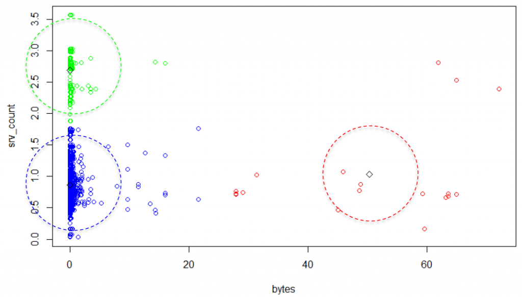
In illustration 2 you can see a very simple two-dimensional example clustering of some sample firewall connections. The x-axis represents the total number of bytes and the y-axis the service count.

You can see that k-means was parameterized with k=3. This leads to three different clusters (blue, red, green). One can see that most of the data points are located along the y-axis. Only a few points are distributed and scattered to the right side. So, we can define these spreaded points on the right as anomalies, because there were a lot of bytes in relationship to only a few distinct services in those connections. The next question is: How can we use this clustering model to detect anomalies? There are three basic approaches to use a clustering model for anomaly detection [1]. First, one could determine fixed „good“ and „bad“ clusters. In our example, the red cluster would be the bad cluster while blue and green are good ones. A second approach could be to look at the density of all clusters. Dense and big clusters could be good, while sparse or small clusters could be bad. A third approach is to calculate a global distance threshold. You can see an example threshold in illustration 2 as dashed lines. If a point exceeds this threshold with the distance to its nearest cluster center, it is classified as anomaly. In some explorative experiments, it showed that this third approach was most reliable in finding abnormal connections.

Prototypical implementation

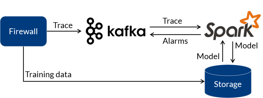
Illustration 3 shows the conceptional architecture for the prototypical application.

All network connections are exported from the central firewall system. This real-time connection trace is sent to a Kafka system. From there it flows to a Spark cluster, where the actual real-time pre-processing and analysis is done. Any alarms are sent back to a separate Kafka topic. From there, e.g. it could be visualized in a dashboard or used to trigger some actions. For model building purposes all the data is also collected and stored in a blob storage. The model is built with Spark MLlib, stored in the blob storage and then used by another job for the actual real-time detection. Illustration 4 shows the principal functionality of the real-time detection job.

Once the model is built and loaded into Spark, an incoming data instance just has to be transformed into its corresponding feature vector. This vector is fed into the clustering model, where a cluster assignment and a distance calculation to the center is made. Now you only need to compare this distance with the pre-assigned threshold.

Some example anomalies

In the following you can see two examples which were detected in the prototypical test phase of the application. The first one in listing 2 shows a typical point anomaly. This means the point itself is classified as abnormal traffic.

The combination of multiple circumstances has led to this alarm. First, this connection has a very unusual port combination of 0/0 which is rare. Furthermore, the transport protocol ipv6-crypt is not a transport protocol at all (usually you have TCP, UDP and ICMP). In addition, this flow contained a very large number of bytes. In fact, this connection was a remote server installation with the system configuration tool Puppet which was done from outside the company network via an encrypted connection. It was the very first time such an installation was done.

The second connection instance is a good example for a collective anomaly. This means that the data point itself would not be classified as anomaly but in collective with multiple similar instances they would be detected as unusual traffic pattern. Have a look at listing 3:

We see an everyday DNS call, characterized with source port 53, transport protocol UDP and exactly one packet. But this exact connection appeared several thousand times in only a few seconds. So the host count, like the service count feature described above, increased more and more while lots of requests were made to the same host, until the data point exceeded its distance threshold in the model.

Conclusion and further reading

We showed how you can build a real-time intrusion detection system based on modern Big Data technologies even with very simple machine learning algorithms like k-means. This post described some basics of feature engineering, required pre-processing steps, possible approaches for anomaly detection with a clustering model, and a high-level overview of the implementation with the help of Spark, Spark streaming and MLlib. In part 2 which will come out soon, we will cover some more advanced algorithms and approaches for anomaly detection in more detail.

Until then, have a look at our Big Data Platforms portfolio and learn more about our Data Science projects!

• [1] Chandola V.; Banerjee A. und Kumar V. (2009): Anomaly Detection: A Survey. ACM computing survey (CSUR), 41 (3). S. 15.
• Slides from the Offenburg Business Analytics Day (German)