The Mystery of Entropy: How to Measure Unpredictability in Machine Learning

If you are dealing with Statistics, Data Science, Machine Learning, Artificial Intelligence or even general Computer Science, Mathematics, Engineering or Physics, you’ve probably come across the term Entropy more than once. Entropy is a significant, widely used and above all successful measure for quantifying inhomogeneity, impurity, complexity and uncertainty or unpredictability. The concept of entropy is more than 200 years old, and still, or perhaps because of that, it is an integral part of the latest machine learning models that are successfully deployed on real-world data sets. In this article, I want to highlight the simplicity, beauty and meaning of entropy.

Entropy and its special forms are able to achieve a conceptual understanding of the data in an intuitive way—something we should exploit more often.

Entropy: What was that again?

I remember countless times that I read something about ‘entropy’, and I asked myself equally countless times  ‚What was that again?‘. So I asked Google for the hundred and first time. Google—once again—threw out a definition of entropy in thermodynamics with which I (as a mathematician) could not do anything and maybe I did not want to. If you want to understand the concept of entropy, information theory is probably one of the simplest approaches. Later we will see that this approach is absolutely compatible with the statistical-mathematical as well as physical concept of entropy.

Let’s start with an information-theoretical view. Everyone knows that a computer is counting on bits. We can ask ourselves ‘how many bits does the computer require to display or transmit information, e.g. a string of characters?’ If the computer needs few bits, the message seems to be less complex. If the computer needs many bits, the message has a high complexity.

Shannon-Entropy

Let’s suppose we’d like to encode the Latin alphabet including some separators and punctuation marks \(X=\{a,b,c,…,z,  `‘  .  ,  ;  !  ?\}\) in bits for displaying them on the screen. In the following figure we consider a tree in which every single character is coded by a sequence of bits. To encode all \(n=32\) characters we need sequences of \(\log 32=5\) bits each: \(a = 00000\), \(b = 00001\), \(c = 00010\), etc.

Well, we can interpret the display of a character as a statistic event. Each event occurs with the same probability. The minimum number of bits needed to display a character can therefore also be formulated as its statistical significance:

\(\log(n) = \log \frac{1}{p_i} = \log(1) – \log(p_i) = -\log(p_i)\) .

At this point, I refer to the information-theoretical (left side of the equation) and statistical (right side of the equation) coherence and it becomes clear what the words ‘inhomogeneity’ or ‘impurity’ have in common with ‘uncertainty’ or ‘unpredictability’.

Characters or events do not always have to be uniformly distributed. In every language there are characters, like the ‘e’, ‘a’ or ‘space’, which appear more frequently than other. For non-uniformly distributed characters we are interested in the expected number of bits to display a message, which can be determined by

\(H((p_1,p_2,…,p_n))=E(-\log p_i)= -\sum_{i=1}^{n} p_i \log p_i .\)

This is what we finally call entropy. It’s nothing new and was defined in 1948 by Claude Elwood Shannon, an US mathematician, electrical engineer and ‘father of information theory’. It is therefore often called Shannon entropy and in literature referred to as

\(H((p_1,p_2,…,p_n))= H((P(X=x_1),P(X=x_2),…,P(X=x_n )))=: H_X\)

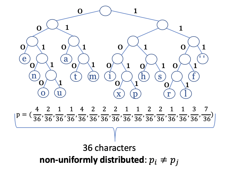
The entropy is maximised if all the characters are equally distributed. That means that the uncertainty is greatest. If we know that some events are more likely than others, we should exploit this in our coding scheme. Imagine that we want to code the sentence ‘this is an example for a huffman tree’. We would like to allocate fewer bits to frequent characters than characters that are rare. An optimal coding scheme as in the figure below can be found by the huffman coding, named after David A. Huffman.

In the picture above the distribution of the letters in the sentence was used for the sake of simplicity. Usually one would use the distribution of the characters over many documents or a general estimated distribution of the characters in German texts. For optimal coding, the probability of \(1\) and \(0\) is exactly \(0.5\).

Cross entropy

We talked about the distribution of the character frequencies in a language. Each language has its own distribution of characters and a corresponding optimal code. However, the code for the English frequency distribution will not match the German frequency distribution. The cross entropy is the expected number of bits per message needed to encode events drawn from a true distribution \(q\), if using a code for distribution \(p\) rather than \(q\):

\(H_X (p,q) ≔E_q (-\log p(x)) = -\sum_{x \in X} q(x) \log p(x).\)

Kullback-Leibler-Divergence

The relative entropy or Kullback-Leibler-Divergence is the expected number of extra bits per message needed to encode events drawn from true distribution \(q\), if using a code for distribution \(p\) rather than \(q\):

\(KL(p,q) ≔-\sum_{x \in X} q(x) \log \frac{p(x)}{q(x)}.\)

Note that \(KL(p,q)\) asks for extra bits, while \(H_X(p,q)\) asks for total bits. It is \(H_X(p,q)=H_X(q)+KL(p,q).\)

Conditional Entropy

Finally the question arises, what can we say about the entropy of an event \(X\), if we already know the previous event \(Y\). In other words, conditional entropy measures the uncertainty of a message generated by source \(X\) after we know that event \(Y\) has generated another message. If \(Y\) can functionally determine the value of \(X\), it is worthwhile that the conditional entropy \(H_{X|Y}\) is \(0\). On the other hand \(H_{X|Y}\) is \(H_X\), if the events \(X\) and \(Y\) are stochastically independent. Let’s suppose we know the conditional probabilities \(p(x|y)\),

then the conditional entropy is given by the entropy of the conditional probabilities, weighted by the probabilities of the previous event \(Y\):

In formula it is \(Η_{X|Y} ≔-\sum_{y \in Y} p(y) \sum_{x \in X} p(x|y) \log p(x|y)\). One can show that \(H_{X|Y}=H_{X,Y}-H_Y\). Assuming that the combined system determined by two messages \(X\) and \(Y\) has a joint entropy \(H_{X,Y}\), the total uncertainty is reduced if we know the event before.

More Entropies

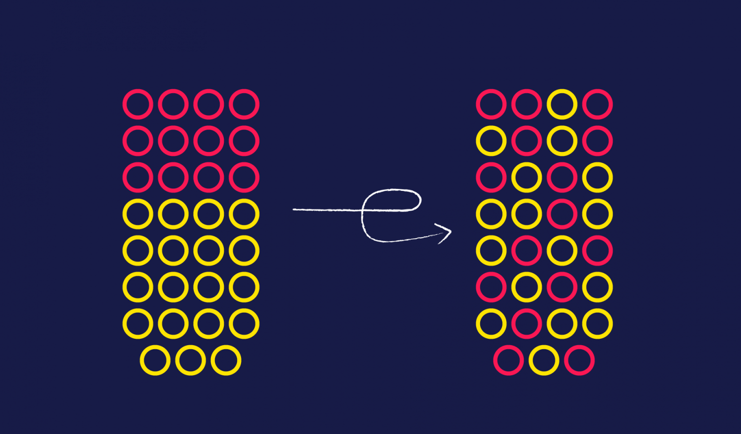
Of course, there are numerous extensions and modifications of entropies that can’t all be dealt with in this article. In addition to information theory and statistics, entropy is also used in thermodynamics and fluid dynamics, where it does not refer to data, but to the distribution of temperature, gas or liquid mixtures. Look at a glass of KiBa (German abbreviation for cherry-banana juice). We all know the moment when the waiter/waitress brings a glass to the table—the lower half of yellow banana juice, exactly separated from the top with red cherry juice. At home, when we mix a glass of KiBa ourselves, it resembles a brown mixture. The waiter’s/waitress’ glass has a low entropy, a high degree of homogeneity or purity. We can say with great certainty that there is a banana particle next to another banana particle. Our glass at home, however, has a high degree of inhomogeneity or impurity.

Power of Entropy in Machine Learning

Having discussed the theoretical concept of entropy in information theory, statistics, and physics, entropy is used successfully in real-world applications in machine learning.

Classification with Logistic Regression or Neural Networks

Cross entropy is the standard loss function for logistic regression and neural networks. Let \(p\) be the true distribution (i.e. the distribution of the training set), and let \(p̂\) be the distribution described by a model. For a classification model modeled by a binary logistic regression model, we have class \(0\) and class \(1\). The model assigns to each input \(x\) the probability that the output \(y\) is in class \(1\), written as: \(p̂(x)=P(y=1|x)= ŷ\). It is \(P(y=0 | x)= 1-ŷ\). Logistic regression learns by minimizing a loss function. Intuitively, we want to assign more penalty if \(1\) is predicted, while the true value is \(0\) and if \(0\) is predicted, while the true value is \(1\). We achieve this by the loss function:

$$ Loss(y,ŷ)=\begin{cases} -\log(ŷ) & \textrm{ if } y=1 \\ -\log(1-ŷ) & \textrm{ if } y=0 \end{cases} $$

Summation over all n training data samples yields to

$$ -\frac{1}{n} \sum_{j=1}^{n} ŷ_j \log(ŷ_j)+(1-y_j) \log(1-ŷ_j).$$

We get by definition the cross entropy between empirical and estimated distribution

$$ -\frac{1}{n} \sum_{j=1}^{n} \sum_{i=1}^{n} p_i \log(p̂_i) + (1-p_i) \log (1-p̂_i)=H(p,p̂).$$

Artificial neural networks are closely related to logistic regression. Basically, logistic regression is a single-layer neural network with the sigmoid function as activation function. One of the greatest features of logistic regression is that the logistic loss function is convex, so we are guaranteed to find the global minimum. Therefore, the cross entropy is preferable to other loss functions.

Decision Trees

Decision trees are classification or regression models in the form of a tree structure. They decompose a dataset into smaller and smaller subsets, while simultaneously developing an associated decision tree incrementally. For example, the popular ID3 algorithm from 1985 minimizes the information gain \(H_{X}-H_{X|Y}\) to calculate the homogeneity of a dataset. In order to divide the training dataset into homogeneous groups, the minimum is achieved in stepwise splits, if all observations belong exclusively in one of the two classes. Decision trees in machine learning are often dismissed as ‘old AI’, yet they still make a significant contribution to the success of innovative algorithms. On the platform Kaggle, owned by Google LLC, Data Scientists, Machine Learning Engineers and other interested scientists meet for competitions on real-world data sets to face the challenges of artificial intelligence and to build best algorithms. Many winners’ solutions comprise XGBoost, an implementation of the Gradient Boosted Decision Trees algorithm. Gradient boosting generates a predictive model in the form of an ensemble of weak predictive models, typically decision trees. Like other boosting methods, it builds up the model step by step and generalizes it by enabling the optimization of a differentiable loss function. For the reasons mentioned above, cross entropy is a good choice as loss function.

Achieving a Conceptual Understanding of the Data

As we have seen, many machine learning and deep learning models successfully use different kinds of entropies as part of their loss functions to train their parameters. We do not need to talk about deep neural networks being able to do amazing things. They do! But the word ‘deep’ in deep learning refers to a technical, architectural property rather than a conceptual one. Deep neural networks are usually quite complex and contain a variety of parameters that can be optimized across multiple levels of interaction. The problem with such black boxes is the lack of trust and interpretability my colleague Marcel Spitzer deals with in another blog post. One can not explain the decision of the model by merely consider its internal elements.

In particular deep neural networks learn a representation of their input data in the hidden layers, e.g. via activation functions. Each (hidden) layer have an (own) activation function as the identity, sigmoid function, tanh, ReLU, Softmax-function or many others. They can be linear or non-linear. Non-linear activation functions make the network especially powerful. This representation is then subsequently used for classification or regression in the output layer. If you want to learn more about deep neural networks, read the blog post of my colleague Patrick Schulte.

Activation functions transform the data, but often don’t take into account the intrinsic structures or complexity of the data. Here’s the chance for entropy in representation learning, representing the structure, complexity and inner nature of data. In particular, for sequential data, such as time series or natural language, entropy can be a valuable feature.

Read on

Take a look at our data science portfolio and many exciting case studies from our AI consulting projects, where we implement machine learning models scalable and maintainable to daily business.

If you are looking for new challenges, you might also want to consider our job offerings for Data Scientists, ML Engineers or BI Developers. For students, we also offer internships, supervision of bachelor’s and master’s theses or working student positions on exciting and challenging topics.