Notice:
This post is older than 5 years – the content might be outdated.
Recently, Machine Learning (ML) models have been widely discussed and successfully applied in time series forecasting tasks (Bontempi et al., 2012). In this blog article we explain an exemplary process of how time series forecasting tasks can be solved with machine learning models, starting with the problem modeling and ending with visualizing the results by embedding the models in a web app for demonstration purposes. To illustrate this process we use a real-world example: forecasting ride-hailing demand based on historical bookings.
Ride-hailing is a new form of On-Demand Mobility (ODM), where a customer can digitally hail a ride via a mobile application. Common examples for ride-hailing services are Uber or Lyft. Offering a service that is both cost effective and of high quality for the customer requires the efficient addressing of the supply- demand disequilibrium, which can be alleviated by accurately predicting passenger demand.
In the following we will first explain how to model the forecasting problem and then describe how embedding the models in a web app can be helpful to communicate and assess the forecasting results.
Problem Modelling
Our given data set contains historical bookings where each entry relates to a unique booking of the service, containing, among other information, a booking time stamp.
In our concrete use case we aim to forecast the next 168 hours of demand. Hence we first have to transform the time series data to represent an hourly basis. After cleaning and aggregating the data the result is a time series of the format:
| dateindex | trips |
| 2017-08-09 00:00 | 141 |
| 2017-08-09 01:00 | 75 |
| 2017-08-09 02:00 | 42 |
| … | … |
| 2017-08-09 20:00 | 253 |
| 2017-08-09 21:00 | 245 |
| 2017-08-09 22:00 | 190 |
An autocorrelation analysis on this data (a measure of the internal correlation within a time series) shows the correlation between the demand of successive hours. The correlation is particularly strong for the preceding hour (t-1), the same hour on the days before (e.g. t-24) and the same hour on the same day in preceding weeks (e.g. t-168).

To be able to use our time series data to train our ML models we first have to transform it into a supervised learning problem (more precisely, a regression task). More formally spoken, we can do so by creating an input data matrix \( X \) as a \( [(N-n-h) \times n] \) matrix and the output matrix \( Y \) as a \( [(N − n − h) × h] \) matrix, where \( y_i \) represents the observation value in a certain hour, \( N \) is the total number of observations, \( n \) is the number of previous values to be considered as input features and \( h \) is the forecasting horizon:
\(\begin{equation}X = \left[\begin{array}{l l l l}y*{1} & y*{2} & \dots & y\_{n} \\y*{2} & y*{3} & \dots & y\_{n+1} \\\vdots & \vdots & \vdots & \vdots \\y*{N-n-h} & y*{N-n-h+1} & \dots & y\_{N-h} \\\end{array}\right]\end{equation}\)
\(\begin{equation}Y = \left[\begin{array}{l l l l}y*{n+1} & y*{n+2} & \dots & y\_{n+h} \\y*{n+2} & y*{n+3} & \dots & y\_{n+h+1} \\\vdots & \vdots & \vdots & \vdots \\y*{N-h+1} & y*{N-h+2} & \dots & y\_{N} \\\end{array}\right]\end{equation}\)
With \( h = 168 \) and \( n = 168 \) the resulting data frame looks as follows:
| trips(t-168) | trips(t-167) | trips(t-166) | … | trips(t-1) | trips(t) | … | trips(t+167) |
| 143 | 117 | 204 | … | 125 | 156 | … | 38 |
| 117 | 204 | 169 | … | 156 | 110 | … | 42 |
| 204 | 169 | 51 | … | 110 | 158 | … | 67 |
| … | … | … | … | … | … | … | … |
| 145 | 218 | 113 | … | 133 | 106 | … | 312 |
| 218 | 113 | 280 | … | 106 | 119 | … | 241 |
| 113 | 280 | 177 | … | 119 | 43 | … | 262 |
We can now use this data to train our ML models. If we use a model that natively only supports a single-step output (like a Linear Regression) we have to choose an appropriate forecasting strategy (see Taieb et al. (2012)). In our example we use a direct multi-step forecasting strategy. In the direct multi-step forecasting strategy, every step in the forecasting horizon is predicted independently. In other terms, \( H \) steps are predicted using \( H \) models \( f_h \):
\( \begin{equation}\hat{y}_{N+h} = f_{h}({y*N, \dots, y*{N-d+1}})\end{equation}\)
Ride hailing demand appears to be influenced by various factors, such as time, price for the service or weather. Considering this data as additional input features can improve the forecasting accuracy.
To evaluate the forecasting performance and to find robust models it is important to choose an appropriate evaluation strategy. To take into account the special characteristics of the time series, we, for example, have chosen a sliding window evaluation with a fixed window size (further reading: Tashman, L. J. (2000)).
Assessing the Forecasting Performance
Many data science projects involve multiple stakeholders that not necessarily have the same technical background. Assessing different evaluation metrics for instance might result in confusion about the concrete meaning and implication of a certain figure. One possible way to communicate and visualize the forecasting results is to build a “clickable“ demonstrator app that incorporates the ML models.
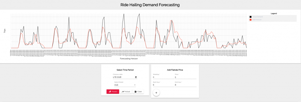
In our case, we built a web app consisting of a backend written with Flask that incorporates the trained ML models (we use scikit-learn for model building) and an Angular frontend to show the predictions. The app allows to pick a certain date and choose an ML model which then forecasts the next 168 steps of demand. The forecast (red line) can then be compared to the actual demand (black line) as shown in the next figure:

To take this a step further, it is also easy to add certain “simulation features“. For example, we can use the demonstrator to show the influence of different pricing strategies. If we exemplarily simulate a flatrate price for the first five days of the week, we see an increase in the overall demand. The black line represents the prediction of an XGB model without a simulated price, the red line represents the prediction under consideration of the simulated price.

Summary
Based on the concrete example of forecasting ride hailing passenger demand, we showed in this article how time series forecasting can be done using ML models. To do so, we first have to transform the time series data into a supervised learning setting and model the demand as a multi step forecasting problem. We find that using ML in this task is a good approach especially due to the the simplicity of considering other (external) features. Furthermore, embedding the ML models in an interactive app proves to be a good way to communicate results and demonstrate different aspects like the influence of a certain input feature on the forecast.
Literature
- Bontempi, G., S. B. Taieb, and Y.-A. Le Borgne (2012). “Machine learning strategies for time series forecasting.“ In: European Business Intelligence Summer School. Springer, pp. 62–77.
- Tashman, L. J. (2000). Out-of-sample tests of forecasting accuracy: an analysis and review. International journal of forecasting, 16(4), 437-450.
- Taieb, S. B., Bontempi, G., Atiya, A. F., & Sorjamaa, A. (2012). A review and comparison of strategies for multi-step ahead time series forecasting based on the NN5 forecasting competition. Expert systems with applications, 39(8), 7067-7083.


Would there be any fundamental problems with combining ML models and show the results of the ensemble instead of letting them choose between models?
Hi Patrick,
thank you for your question. In general, there are no problems at all to combine the ML models to an ensemble. Instead of manually choosing a specific model for a forecast, we could easily use multiple models in parallel (see Bagging) or in a sequence (see Boosting) and only show these results. In our demonstration case however, we specifically wanted to compare the individual models and hence added the option to choose a certain model.
Regards,
Constantin
Awesome. OK thanks so much. That was helpful! I was looking at it more from a business-user pov with zero affinity to technology (there are many). Many non-digital people (typically running traditional companies) get cognitive overloads fast. Maybe they just want ONE graph, showing „the best option“ with „the most wisdom“…? I mean if it’s self-service. In a presentation it’s easier ofc to show options? Have you run into these kinds of situations? Or what worked for you?
That depends on the purpose of the demonstrator. We used the web app for internal evaluation purposes and hence wanted to compare different models. But if the goal for instance is to show the final results of the evaluation process (e.g. the model that finally would be used in a productive system) by using a prototype web app then it might make sense to only show the output of the best performing model without any options.
I have come across a number of works and articles online that make make multiple forecasts on the unseen test data not exactly following a direct or recursive approach but rather a lazy application of an ML model.
What I mean is, they produce features such as data-time, maybe a lag (the same size as the forecast horizon) and time series features other than the target which are all easily available for the unseen future. They then simply feed the data into an ML model and make multiple forecasts/point predictions for the future time steps.
Is that also formally a method of direct multiple forecasting? even though we technically only have one model?
In this case how do we call it?
Thanks for your help in advance.