Notice:
This post is older than 5 years – the content might be outdated.
This is the second part of our series about Machine Learning interpretability. We want to describe LIME (Local Interpretable Model-Agnostic Explanations), a popular technique to explain blackbox models. It was proposed by Marco Tulio Ribeiro, Sameer Singh, and Carlos Guestrin in their paper Why Should I Trust You? Explaining the Predictions of Any Classifier, which they first presented at the ACM’s Conference on Knowledge Discovery and Data Mining in 2016. Please check out our previous article if you are not familiar with the concept of interpretability.
We previously made a distinction between model-specific and model-agnostic techniques as well as between global and local techniques. LIME can be classified as a model-agnostic technique with a local scope. In other words, it enables us to explain particular predictions of any model. In contrast to the techniques described in the first article, LIME is even applicable to models for text and image classification.
What is LIME?
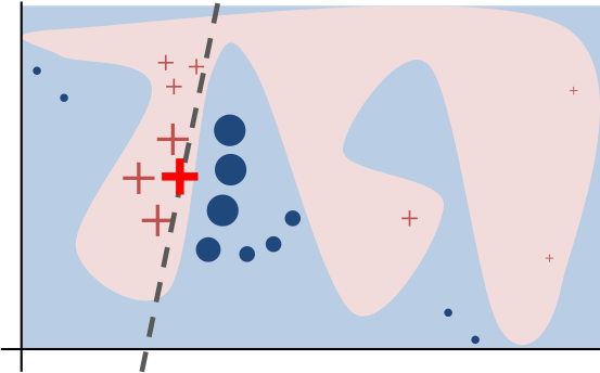
The idea behind LIME is to approximate a complex model locally by an interpretable model and to use that simple model to explain a prediction of a particular instance of interest. It’s comparable to the Global Surrogate technique, but it differs in the fact that it is based on sampled instances that are weighted by proximity to the instance to be explained. Hence, instead of trying to capture the overall behavior of the model, LIME just attempts to be locally faithful to the classifier. The following image shows the non-linear decision boundary of some complex classifier. LIME fitted a linear model, represented by the dashed decision boundary, to sampled instances. Notice that this simple model mimics the complex model in the vicinity of the instance of interest sufficiently well.

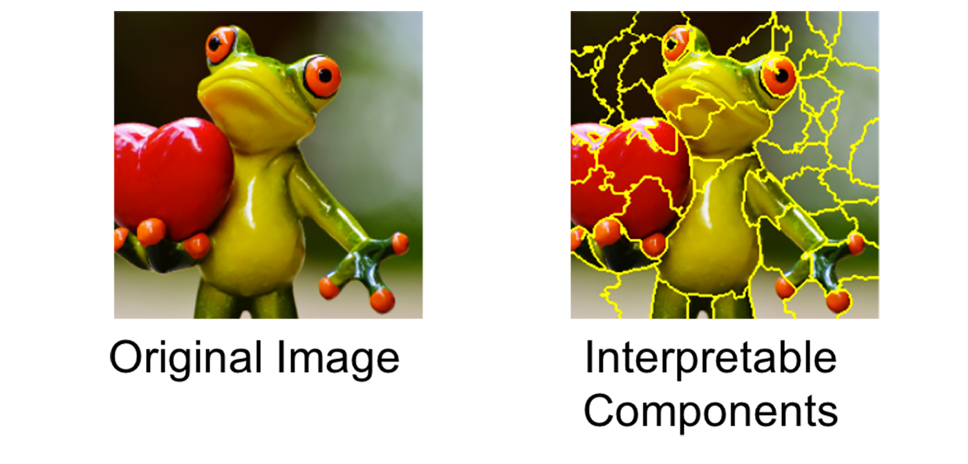
Unlike other interpretability techniques, explanations that are generated by LIME are based on so-called interpretable components which can completely differ from the input features of the original model. Basically, interpretable components are representations of the underlying data which are understandable to humans. For example, an interpretable component can be a subset of words of a text corpus or a contiguous region of an image. The concept of interpretable components enables LIME to be generalizable to high dimensional domains like text or image classification.
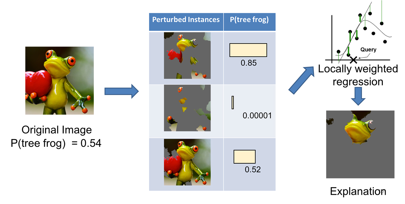
Whatever type of model you try to explain with LIME, you have to think about appropriate ways to determine interpretable components. Common approaches are the bag-of-words model for text classification or pixel segmentation for image classification. Based on that mapping, LIME acts on binary vectors that indicate presence or absence of interpretable components. Apart from that, the original model can be based on much more complex features. It estimates strength and direction of influence for each interpretable component by fitting interpretable models to perturbed instances of those binary vectors. LIME evaluates how perturbations (e.g. removing words of a text, hiding parts of an image) affects the prediction of the original model.

Technically, any interpretable model can be used within the LIME framework. When fitting interpretable models, LIME attempts to balance simplicity and local fidelity. Therefore, a measure of complexity and some locality-aware loss is needed. In most practical cases, sparse linear models, especially The LASSO, perform sufficiently well. The complexity of LASSO models can be measured by the number of non-zero weights. A squared exponential kernel is usually used as a measure of local accuracy.
Now, let’s put it all together to describe each step of the LIME procedure:
- Determine an interpretable representation of the instance of interest
- Draw a sample by disturbing the interpretable representation
- Apply the original model to the perturbed instances
- Fit an interpretable model to proximity-weighted sampled instances and the predictions of the original model
- Use the interpretable model to draw conclusions about the relevance of each interpretable component

How to use LIME?
Enough has been said about the theory behind LIME. Let’s finally use it to explain some predictions. We’ll start with an image classifier:
Image recognition
Let’s import all relevant libraries and a pre-trained Inception-V3 for image classification. Inception-V3 is a deep neural network proposed by Szegedy, et al. (Google) which is composed of 42 layers of roughly 7 million parameters. As described in this LIME tutorial, we cloned the fork of tf-slim and put the pre-trained Inception-V3 into tf-models/slim/pretrained.
|
1 2 3 4 5 6 7 8 9 10 11 12 13 14 15 16 17 18 19 20 21 22 23 24 25 26 27 28 29 30 31 32 33 34 35 36 37 |
import tensorflow as tf import sys import matplotlib.pyplot as plt import numpy as np import os import random sys.path.append('tf-models/slim') slim = tf.contrib.slim session = tf.Session() from nets import inception from preprocessing import inception_preprocessing from datasets import imagenet from lime import lime_image from skimage.segmentation import mark_boundaries random.seed(4711) %load_ext autoreload %autoreload 2 %matplotlib inline |
In addition, let’s define some functions like pre-process and predict:
|
1 2 3 4 5 6 7 8 9 10 11 12 13 14 15 16 17 18 19 20 21 22 23 24 25 26 27 28 29 30 31 32 33 |
image_size = inception.inception_v3.default_image_size def load_image(path): image_raw = tf.image.decode_jpeg(open(path, 'rb').read(), channels=3) image = inception_preprocessing.preprocess_image(image_raw, image_size, image_size, is_training=False) return session.run([[image]])[0][0] names = imagenet.create_readable_names_for_imagenet_labels() processed_images = tf.placeholder(tf.float32, shape=(None, 299, 299, 3)) with slim.arg_scope(inception.inception_v3_arg_scope()): logits, _ = inception.inception_v3(processed_images, num_classes=1001, is_training=False) probabilities = tf.nn.softmax(logits) checkpoints_dir = 'tf-models/slim/pretrained' init_fn = slim.assign_from_checkpoint_fn( os.path.join(checkpoints_dir, 'inception_v3.ckpt'), slim.get_model_variables('InceptionV3')) init_fn(session) def predict_fn(images): return session.run(probabilities, feed_dict={processed_images: images}) |
Now to the image recognition task: We want the classifier to recognize the squirrel in the following image. Let’s see if Inception-V3 is able to spot it:
|
1 2 3 4 5 6 7 8 9 |
squirrel_image = load_image("img/squirrel.png") plt.imshow(squirrel_image / 2 + 0.5) preds = predict_fn([squirrel_image]) for x in (-preds).argsort()[0][:3]: print(x, names[x], preds[0,x]) |

Actually, the Inception net is quite sure that there is a fox squirrel in the image. Pretty impressive!
Now, that we observed the outcome of our complex classifier, let’s apply LIME to identify parts of the image having most influence to the squirrel prediction. To do this, we feed an explainer with the squirrel image and provide it the number of patches to be determined (num_features) along with the number of perturbations of the interpretable representation (num_samples):
|
1 2 3 4 5 6 7 8 9 10 11 12 13 14 15 |
explainer = lime_image.LimeImageExplainer() explanation = explainer.explain_instance( image=squirrel_image, classifier_fn=predict_fn, top_labels=1, hide_color=0, num_features=20, num_samples=500) |
Ok, let’s see which parts of the image accounted most to the squirrel prediction:
|
1 2 3 4 5 6 7 8 9 10 11 |
masked_image, boundaries = explanation.get_image_and_mask( label=336, positive_only=True, num_features=6, hide_rest=True) plt.imshow(mark_boundaries(masked_image / 2 + 0.5, boundaries)) |

It was the squirrel’s face and its bushy tail. Both, quite reasonable causes for the squirrel prediction. Well done, Inception!
Tabular data
LIME is not only applicable to image data. We can also use it to explain predictions that are based on tabular data. As biology teaches us, squirrels are mammals. Let’s find out whether a neural net classifier is able learn and predict this, too. We therefore train a multi-layer perceptron on the Zoo Data Set, a small tabular dataset in which various species are categorized into seven classes based on 16 different features:
|
1 2 3 4 5 6 7 8 9 10 11 12 13 14 15 16 17 18 19 20 21 22 23 24 25 26 27 28 29 |
import pandas as pd from sklearn.model_selection import train_test_split from sklearn.neural_network import MLPClassifier from lime import lime_tabular classes = ["mammal", "bird", "reptile", "fish", "amphibian", "bug", "invertebrate"] df = pd.read_csv("zoo.data", header=0, sep=",") squirrel = df[df.name == "squirrel"] df = df[df.name != "squirrel"] X_train, X_test, Y_train, Y_test = train_test_split(df.drop(["type"], axis=1), df.type) X_test = pd.concat([X_test, squirrel.drop(["type"], axis=1)]) Y_test = pd.concat([Y_test, squirrel.type]) X_test_names = X_test.name X_train.drop("name", axis=1, inplace=True) X_test.drop("name", axis=1, inplace=True) clf = MLPClassifier(alpha=0.25, hidden_layer_sizes=(25,)).fit(X_train, Y_train) |
We imported all necessary packages, loaded the dataset and did some preprocessing on the data such as removing the observation for the squirrel from the train dataset. Finally, we trained the neural net on 75% of the original dataset.
Now, let’s see which class the classifier assigns to the squirrel:
|
1 |
print(pd.DataFrame(clf.predict_proba(squirrel_features), columns=classes).transpose()) |

As we can see, the classifier assigns the highest probability of 88.1% to the mammal class, which is actually correct. Nice!
But why does the model decide upon the mammal class? Since the neural network is a complex, non-linear model, it is difficult for us as humans to understand the model’s decision process. Yet, we can leverage LIME to support us in comprehending its decision. Let’s have a look at the LIME estimate of relevant features for the squirrel prediction:
|
1 2 3 4 5 6 7 8 9 10 11 12 13 14 15 16 17 18 19 20 21 22 23 24 25 |
explainer = lime_tabular.LimeTabularExplainer( X_train.values, categorical_features=[0,1,2,3,4,5,6,7,8,9,10,11,13,14,15], feature_names=X_train.columns, class_names=classes, discretize_continuous=True ) exp = explainer.explain_instance( squirrel_features.values[0], clf.predict_proba, num_features=16, top_labels=1 ) exp.show_in_notebook(show_table=True, show_all=False) |
We took the calculated class probabilities and list the impact of all features (16 in total) for the top class. In that particular case, the class is mammal.
The graph below shows the estimated impact of each feature. Bars starting in the middle and expanding to the left (colored in turquoise) decrease the probability of the instance in question to belong to the class mammal. Bars in blue expanding to the right increase the predicted probability that the squirrel is a mammal. We can see that most features had a positive contribution to the probability of the mammal class.

For example, the fact that a squirrel gives milk to feed its offspring and that it is not venomous are plausible explanations, and it makes sense that these two facts had a positive contribution to the final prediction. Furthermore, the length of a bar indicates the magnitude of the feature’s influence. Thus, giving milk, having fur and not laying eggs are the most influential or rather most discriminative features for a squirrel being a mammal.
Conclusion
While most of the techniques that were described in the first blog post are global techniques, LIME is a technique that has a local scope. Therefore, LIME allows us to explain particular predictions of any classifier. The LIME framework is flexible in the sense that any interpretable model can be used to explain predictions. Furthermore, the concept of interpretable components enables LIME to be applicable to high dimensional domains such as image or text classification. Overall, LIME can be used to support model selection and to generate trust by reviewing expressive examples.
Read on
You might wanna have a look at our deep learning portfolio. If you’re looking for new challenges, you might also want to consider our job offerings for Data Scientists, ML Engineers or BI Developer.


