Data processing scaled up and out with Dask and RAPIDS (3/3)

This blog post tutorial shows how a scalable and high-performance environment for machine learning can be set up using the ingredients GPUs, Kubernetes clusters, Dask and Jupyter.  In the preceding posts of our series, we have set up a GPU-enabled Kubernetes platform on GCP and deployed Jupyterhub as an interactive development environment for data scientists. Furthermore, we prepared a notebook image that has Dask and Dask-Rapids installed. Now it is time to actually do some coding and compare the results. In this final article, we will compare the efficiency of four approaches for a typical machine learning task: a random forest. We will implement it in Sklearn, which uses only one machine (and 2 cores), then we will parallelize the Sklearn code with Dask, and execute it on up to 4 machines (each with 2 cores). Finally, we will use the GPUs: a single one with Rapids and multiple with Dask-Rapids.

We can access JupyterHub on port 8000 from the browser, log in (if authentication is enabled) and we can see the workspace of our JupyterLab instance.

For evaluation, we will take a look at the Dask-Rapids example, load a dataset and fit a Random Forest to it. After that, we will compare the performance between Sklearn (single-Node CPUs), Dask ML (multi-Node CPUs), cuML (single GPU) and Dask-cuML (multi GPU).  About the dataset: We will use a real case dataset from the Santander Bank (customer-transaction-prediction) which is a 300MB .csv file.

Sklearn

Let’s start with the Sklearn example. We load the dataset with Pandas, split the dataset into train and test (80/20) and specify the parameters for the forest. After that, we can start the fit function, wait until it is done and then make predictions for the verification part. Finally, we can take a look at the score. The code and results:

An important aspect here is the n_jobs  parameter (the number of available cores, in our case: 2) in the specification of our forest. With Sklearn, you can use all the cores of a single machine to speed up computing. But it would be neat to use more than a single machine has to offer – for example to combine the cores of all the nodes in our cluster. This is where Dask comes into play.

Dask

Dask offers the possibility to easily parallelize the code we used above across the whole cluster. Actually, the only changes we have to apply is to persist the data across the workers and wrap the fit function with the joblib.parallel_backend function. Specification for the workers needs to be defined and GCSFS needs to be present on the workers as well, hence it is added under extra pip packages. This is how it looks in this case:

The image parameter defines the registry where the image can be pulled from. One can use the official and up-to-date image daskdev:latest. Although the components of our base image with Cuda, Dask and Rapids are updated regularly and frequently, it may be a little bit behind. To avoid inconsistencies between the client (scheduler – Jupyter) and the workers we built an image for the workers with pinned versions instead. In the worker-spec.yaml we can also specify the resources or extra packages that need to be installed when starting the worker pod. An important part is mounting the config map with credentials to access the Bucket by setting the Volumes and VolumesMounts parameters. The Dockerfile for the workers can be seen here:

The prepare.sh can be copied from the official dask repository. It needs to reside in the same folder as the Dockerfile for the workers. Prepare.sh:

Let’s take a look at the code and see how much better we can get. First, we will use only one worker, with 2 cores and 6GB of RAM. Then 2, 3 and finally 4 workers:

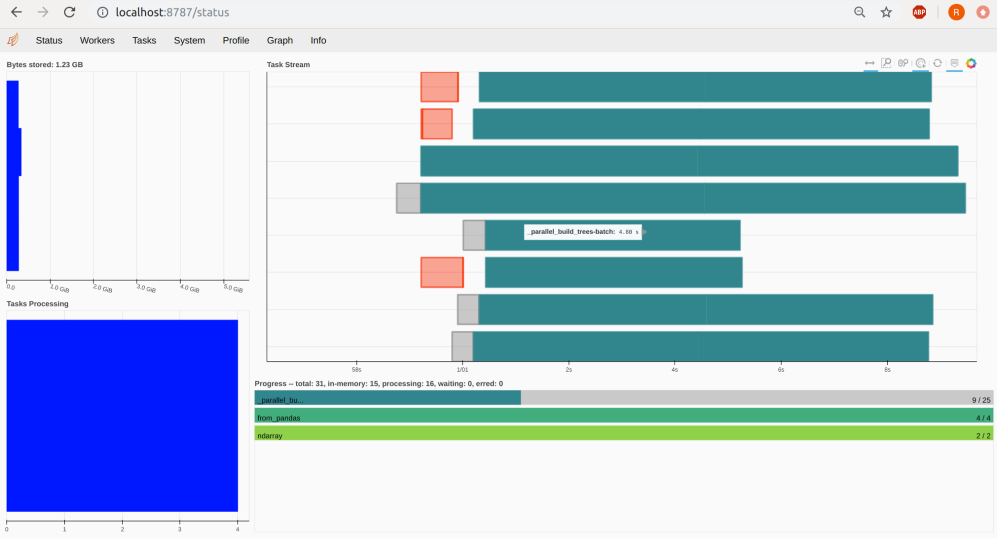
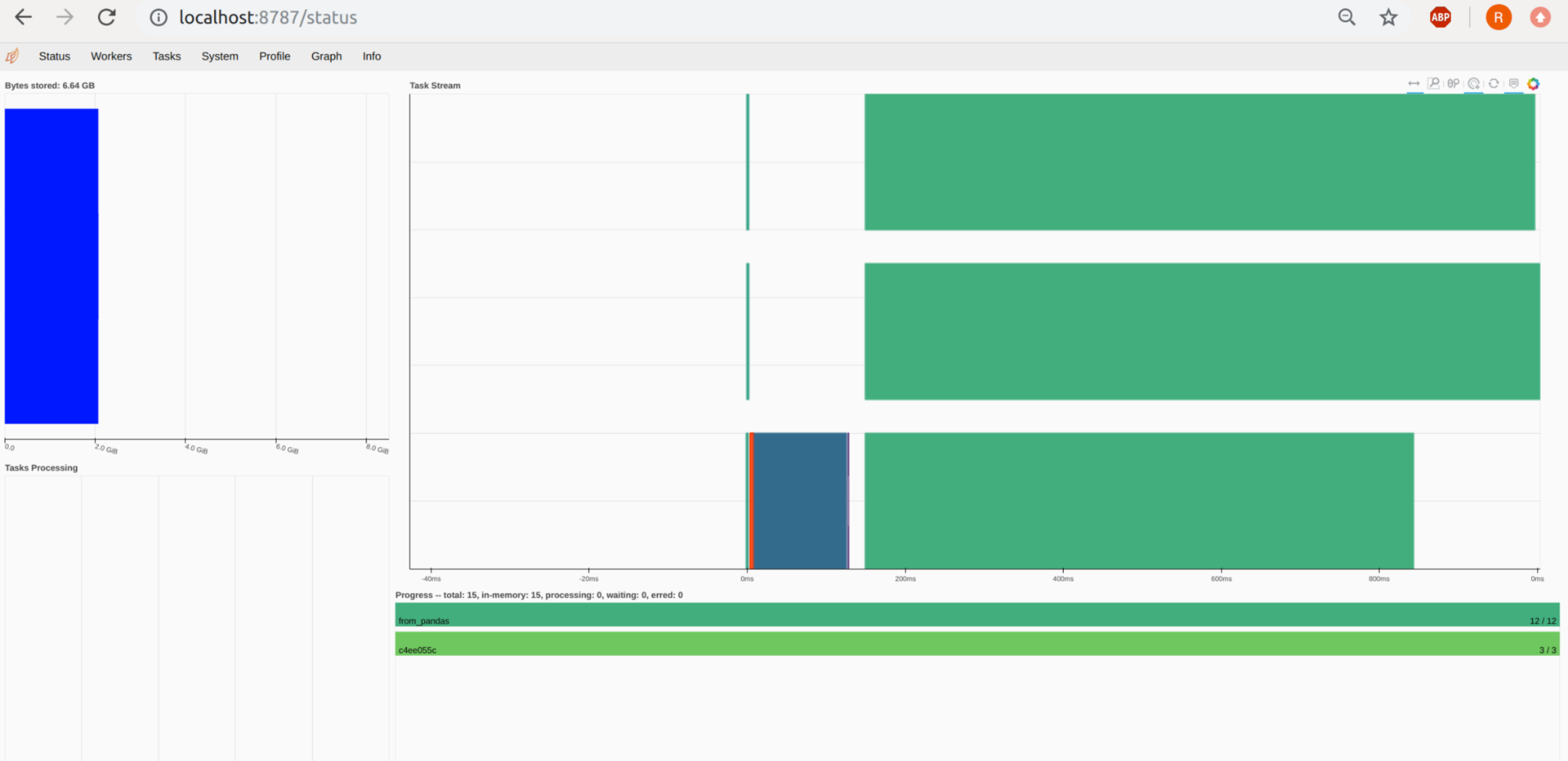
You can port-forward your Jupyter pod on 8787 and see the Dask Dashboard under http://localhost:8787. The workers, their tasks and resources can be viewed there. In the below example you can see 4 workers, with 2 CPUS (Threads) each, hence we see 8 Task Streams:

Rapids – cuML

We have parallelized the Random Forest across the CPUs of our cluster. Now let’s use some GPUs. We start with focussing on one GPU with the RAPIDS cuML library. Since its API is similar to the one of Sklearn, the code will look similar as well. With cuDF we can read the dataset .csv file directly from the bucket. Splitting the dataset into train and test looks almost like in Sklearn. An important thing to keep in mind are the datatypes. Although we can train the Forest with float64 if we want to use GPU-based prediction, we should use float32 for training. Labels should be int32.

Dask-Rapids – cuML

If one GPU is not enough, we can use more of them. With Dask-Rapids there are two possibilities. The first one, which will be shown here, is a Multi-GPU computing which can combine all the GPUs of a certain node. It is done by creating a LocalCUDACluster, which automatically recognizes the GPU’s cluster on the node that runs Jupyter (in this case). For this scenario, no Docker image is needed for the workers simplifying the configuration. The second possibility is multi-GPU/multi-node computing which takes one GPU from every considered node. In this case, similar to the Dask-Sklearn example from above, a specification and an image for every worker is needed.

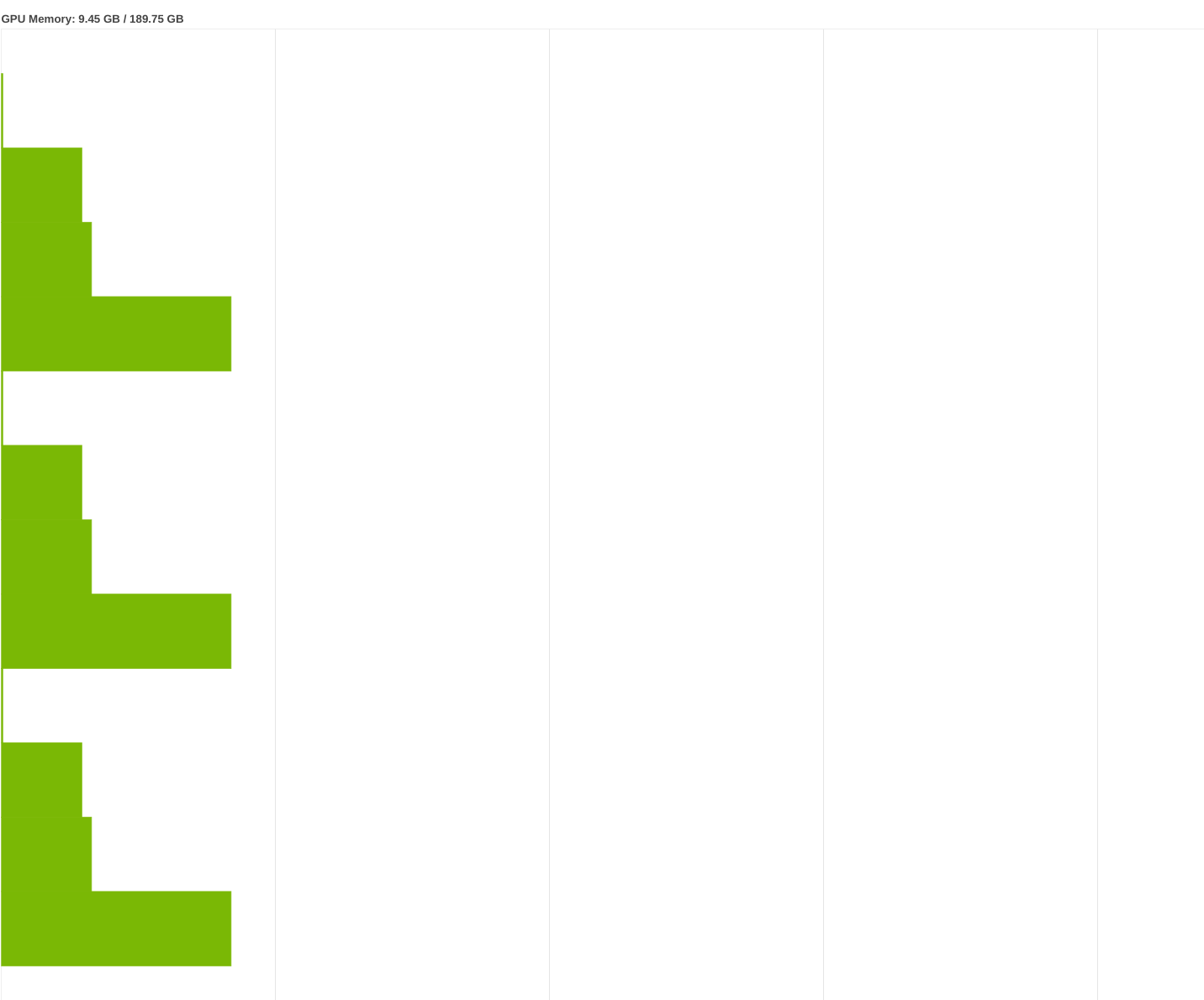
Like said before, we start by creating a LocalCUDACluster(n_workers=n). If we omit the n_workers specification, all available GPUs from our node will be taken. Then we connect to the client. A dashboard is available as well, just like in the Dask-Sklearn example. A little tip for the dashboard: http://localhost:8787/individual-gpu-memory and http://localhost:8787/individual-gpu-utilization show more detailed information about the actual state of our GPUs.

Since Dask-cuDF does not offer splitting the dataset into train and test parts (at least at the time this article was written), we will use the standard cuDF read function, split our dataset, and finally convert it to Dask-cuDF Dataframe & Series. For the convert step, we need to specify how many partitions we want for our data. Choosing a number which corresponds to the number of our GPU workers seems reasonable.

A necessary step is to persist the data across all the workers. Unlike in the Dask-only version, a simple persist is not enough. We need to use the Dask-cuML function persist_across_workers. By this we make sure, all the workers (GPUs) will have access to the data while performing fit or prediction:

Results and Experiences

Sklearn only took about 1min 13sec to fit the forest. Using Dask-only without any GPU, we can speed things up pretty nicely. Using only one worker yields a bit worse results than Sklearn, which is not surprising since costs (computational/administrative overhead) of distributed computing are not to be ignored. However, with every new worker the computation time was decreasing, leading to an almost x2.5 speed-up with 4 workers. The real game-changers are the GPUs. We can observe a x48 speedup with a single GPU compared to Sklearn and almost a x20 speedup compared to Dask with 4 workers.

We can do even better if we use Dask-Rapids and a few GPUs. The difference here is not that spectacular due to the size of the data. At some point, scaling brings no improvement. Even more, adding a 4th GPU would lead to an increase in computation time compared to 2 or 3 GPUs.

An interesting aspect is the prediction time. Here Sklearn clearly wins the fight with a prediction time of 324ms, while single GPU cuML needs about 897ms. Prediction time is even worse if we use distributed GPU computing with Dask-cuML. Here the prediction time was from 6.16s (2 GPU) to 4.44s (3 GPUs). The accuracy, however, was nearly the same at about 89.877% for GPU-based RF and 89.882% for Sklearn.

Troubleshooting

There may be a few problems you will encounter on your way trying to configure everything. Rapids is generally made for GPUs that have a Compute Capability (CC) of 6.0 or higher. So if you want to use, let’s say, a Tesla K80 with CC 3.7, you will not be able to fully use Rapids’ functions and you will encounter the Error no kernel image is available for execution on the device. You can omit that by installing Rapids from source and changing the CC in the CMake file. However, there would not be a 100%-guarantee that everything works as it should.

Other problems may occur while building your own images with Rapids and Dask. You have to keep the dependencies in mind. For example, Rapids (0.13) requires a lower version of Pandas than the one installed with Dask. You have to specify and pin versions. This helps with keeping the Dask-worker image in consistency with the client image.

While deploying JupyterHub, it may take a long time to pull the image from the repository (about 15-20 minutes in my case). That is because the images are pretty big, having CUDA, Jupyter, Dask and Rapids installed. This may result in a timeout error. You can add a –timeout flag with a large number to the deployment command to avoid this.

If you cannot access the Buckets from Jupyter, check whether you (Jupyter + Workers) have the access to the credentials and if the  GOOGLE_APPLICATION_CREDENTIALS variable is correctly set.

Summary

In this blog post series, we have learned a few things. In part 1 we set up a Kubernetes cluster on GCP with accessible GPUs, including installing the chart manager Helm2 (or Helm3). After that, in part 2, we prepared the environment to work with: JupyterHub with proper notebook images – including the CUDA library – with Dask, Rapids and Dask-Rapids on top of that.

Finally, we took a look at a practical use-case for Dask and Dask-Rapids, presenting a Random Forest implementation using 4 different methods. While Sklearn, using a single machine, is the slowest one, it is easily parallelized with Dask, which allows it to use more than a single machine and in the case of 4 workers enables a decent speedup of 2.5x. The real game-changers, however, are the GPUs. Rapids offers a Pandas-like interface and a single GPU increases the performance dramatically, resulting in a 48x speed-up over Sklearn. As if one GPU is not enough, one can use Dask-Rapids to combine several graphic units! But keep in mind, while training is much faster with GPUs, the prediction time is better on a CPU. So, as always, smart design for best efficiency is required.