Sequential Recommender Systems can capture information from a sequence of items in a user history to generate more relevant recommendations. However, the user history is not always strictly sequential. In this article, we will take a look at two models that capture and eliminate noise from user-item interaction sequences.
Traditionally, recommender systems generate recommendations based on the items with which a user has previously interacted. For example, if the user has bought a laptop, it makes a lot of sense to recommend him/her a laptop case or a mouse. But what if we consider not only the last item the user interacted with, but the whole sequence of items in the user history? Then, we will be able to understand the context in which recommendations are made, which can help us to make recommendations more relevant. For example, if the user’s purchase pattern is „eggs — flour — yeast“, recommendation of other baking ingredients will be more relevant compared to the scenario where the user just buys eggs or flour. Capturing information from the ordered sequence of items to generate more relevant recommendations is the main task of Sequential Recommender Systems (SRSs). The underlying assumption of SRSs is that sequences of items are inherently sequential, with each item having a strong influence on its successor. This, however, oftentimes is not the case in real life, where the sequences may contain noisy items that affect the model predictions. In this article, we will take a look at two models that capture and eliminate noise from user-item interaction sequences.
What is noise
Generally, noise is divided into two categories: malicious and natural noise. Malicious noise is produced by an attacker who – for example – deliberately tries to insert false data into the system. Natural noise is produced by the users who may unintentionally introduce noise into data. Some of the major factors that can cause natural noise are are social surroundings, mood, personal conditions, and context.
Natural noise can occur in data due to various domain-specific reasons. For example, in the domain of web personalisation users could make many navigation mistakes (e.g. due to a poor website design) that could significantly lower the prediction quality. In the e-commerce domain, users can search for a present for their friend or can make a spontaneous purchase based on their mood. In the movie/music domain, users may briefly switch their tastes based on the social surroundings (e.g. watching comedies with their family and horror movies with friends). Malicious noise is easier to identify as attackers follow certain patterns. Meanwhile, natural noise is more challenging to capture as there are various reasons causing this noise. In this article, we will consider the models that are able to identify natural noise in item sequences.

An example of natural noise is described in the figure above taken from the research of Yan et al. (2019) (find referenced works at the end of this blogpost). The sequence of items is thematically connected, except for the one unrelated item, which you may guess is the bike, that nevertheless influences the next item recommendation in a sequential recommender. If we eliminate the noisy item from the sequence, the model should yield a better performance by capturing an accurate, undistorted information from the order of items in the sequence.
In the following, we will present, discuss and evaluate two models we created to detect and resolve this problem:
Model I: SRAR
Sequential Recommender with Association Rules (SRAR) is a model that uses a combination of Association Rule (AR) mining with a Deep Learning (DL) technique. The goal of ARs is to uncover relationships between elements of an information repository. ARs consist of antecedent and consequent items, where the latter follows the prior. By identifying an antecedent and consequent correctly, which could consist out of one or multiple items in a database, ARs are able to find closely related items. This means that filtering sequences based on ARs would eliminate items that are not strongly associated with one another. The items with no strong association are assumed to be noisy. Therefore, by capturing and eliminating them, we expect to boost the performance of a sequential recommender.

The model architecture of SRAR is presented in the figure above. The model is composed of three pre-processing blocks: mining of ARs, filtering of sequences, and subsequent padding of sequences. The data is then passed to the pairwise encoding block, and the output is fed into a CNN.
Suppose we have a user \(u\), a user-item interaction sequence of size \(L\), and targets of size \(T\) that the model has to predict. At the pre-processing step, the ARs of size 2 are mined based on the training set consisting of the user-item interaction sequences.
To account for popularity bias, support and confidence are integrated. For an AR, the number of times at which a pair of items \(AB\) occurs in the sequence will constitute support count of the pair. Then, confidence will constitute the percentage of the sequences that contain \(AB\) pair among the sequences that contain only item \(A\). The pairs that achieve the minimum support and confidence threshold are considered pairs with strong dependencies.
Having mined frequent item pairs from the training set, the training sequences are filtered based on the mined ARs. After filtering, only the frequent item pairs are left in the sequence, while infrequent pairs are discarded. The new sequences are then padded to the longest possible sequence. Padding in the pre-processed sequences is represented with a zero vector \(\vec{0} \in\mathbb{R}^D\). Given the original sequence of size \(L\), we get the longest possible sequence \(L\times(L-1)\), which corresponds to the number of all possible pairs of items given a sequence of size \(L\).
For each item \(i\in I\) and user \(u\in U\), an embedding vector of size \(D\) is initialised. The embedding vector is initially sampled from a normal distribution and is iteratively adjusted via backpropagation during the training process. Then for a pre-processed sequence of item pairs, item embeddings and user embeddings are retrieved. The goal of the pairwise encoding block is to capture relationships between non-adjacent items. Rather than applying convolutional layers to the initial input embedding, a three-dimensional (3D) tensor is created to which convolutional layers are then applied. In this way, the model is able to capture relationships not only between the immediate items, but also between the items located in different parts of the sequence. In the 3D tensor, items are stacked against each other, so that all possible pairs of items are considered . An embedding for a \((i,j)\) pair of items is formed via concatenation of embeddings of separate items \([e_i, e_j]\). Note that the pairwise encoding tensor contains the padded pairs (illustrated with a grey hyper-rectangle in the Architecture of SRAR Model) that have no influence on the model prediction. Thus, only frequent item pairs influence the prediction, while infrequent pairs are deactivated.

The obtained feature map, represented by the 3D tensor, is further fed into a CNN.The CNN architecture consists of two convolutional blocks, and each block has two convolutional layers. Each convolutional layer is followed by Batch Normalisation and ReLU activation. The number of channels grows from 128 to 256 between the first and the second convolutional blocks to extract more complex sequential dependencies. Afterwards, the maxpool layer is applied to capture the strongest sequential features. The sequential feature vector \(s\) is obtained by applying a Fully Connected (FC) layer with dropout to the output of the maxpool layer.
To account for a user’s general tastes and preferences, the sequential feature vector \(s\) is concatenated with the user vector \(u\) and projected onto another FC-layer with \(I\) number of nodes to get the final sequence vector. Finally, a sigmoid function is implemented to get independent probabilities of each item being recommended.
Model II: SRAttn
Sequential Recommender with Attention (SRAttn) pursues the same objective: improving recommendation by eliminating the irrelevant items from the user-item interaction sequences. The model, however, utilises a different approach: a CNN with an attention mechanism. The attention mechanism is able to memorise items that lie close to one another in the feature space, assigning higher weights to their corresponding item embeddings while assigning lower weights to the non-related items.

Similarly to SRAR, for each item \(i\) and user \(u\), an embedding vector of size \(D\) is initialised. Then, for each item in a sequence, a tensor of size \(L \times L \times 2D\) is created by stacking pairs of items and their corresponding embeddings. The attention mechanism is then applied to the tensor in order to detect the irrelevant pairs and deactivate them by bringing their embeddings close to \(0\).
The attention mechanism block is implemented based on the scaled dot-product attention introduced by Vaswani et al. (2017). Since there are no arbitrary queries, keys and values in our CNN model, the attention mechanism is applied directly to the pairwise encoding tensor. First, the pairwise encoding tensor of size \(L \times L \times 2D\) is linearly projected onto a tensor with dimension\(L \times L \times 6D\), which is subsequently divided into \(Q, K, \text{and } V\) tensors. Then, the scaled dot-product attention is applied as in the figure below. At this step, the similarity of a pair in a sequence to every other pair in the sequence is measured using the dot product. Pairs of items that are located close to one another in the feature space will get a higher dot product value, which is transferred into a higher weight applied to the tensor \(V\).
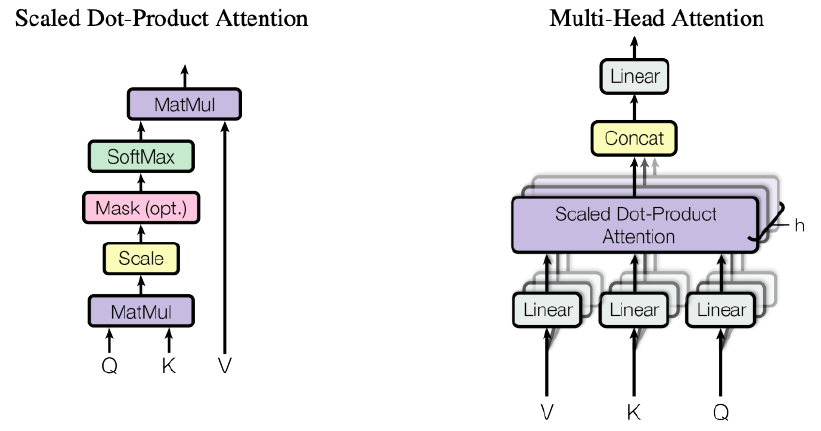
For each head \(h\), the scaled dot product is performed separately to take into account different aspects of items, e.g. for a movie recommendation, it could be movie genre, actors, or budget. Finally, the output of each head is concatenated and projected onto the linear layer, and the resulting tensor with the transformed item embeddings is obtained. Conceptually, the output of the attention mechanism is a transformed version of the original pairwise encoding tensor with its values being adjusted based on the similarity of item pairs, where the irrelevant pairs receive low embedding values and thus are deactivated.
The feature map represented by the transformed tensor is subsequently fed into a CNN to capture high-order relationships among items. The structure of the CNN is identical to the one implemented in SRAR.
Measuring the models‘ ability to capture noise
Performance of the models
To check the ability of the models to capture noise, we evaluate the performance of the models based on three publicly available datasets: MovieLens, Gowalla, and Last.fm. The extent of noise in the datasets has not been quantitatively measured, meaning that it is only implied that the datasets contain noise as user imprecision is highly likely in such big datasets as these.
The metrics used to evaluate the performance of the models are Precision, Recall, and Mean Average Precision (MAP). In this research, we relax the constraint of predicting the next immediate item in the sequence to the next \(N\) items in a sequence. Therefore, Precision and Recall are extended to take the next \(N\) items into account, becoming Precision@\(N\) and Recall@\(N\). In the research, we consider \(N\) of sizes \(1,5, \text{and } 10\).
As a benchmark for the models, a number of baselines are implemented:
- Popular (POP) baseline is one of the simplest baselines, yet it can yield robust results in certain domains. First, the items are ordered based on the frequency of their occurrence. Then, the most popular $N$ items are recommended to every user
- Caser: a CNN-based model for top-N personalized recommendation
- CosRec: a CNN-based model with a pairwise encoding block
- GRU4Rec: a session-based RNN model

The results of the models along with the state-of-the-art baselines are presented in the table above. First, let’s take a look at performance of the baselines. Among the baselines, CosRec yields the best results on all three datasets, highlighting the importance of modelling the relationships between non-adjacent items within a sequence. Popular baseline generates the worst results, signalling the importance of personalised recommendations.
SRAR performs worse compared to CosRec, on the two datasets — MovieLens and Gowalla. This can be explained by the effect of ARs on the model predictions: since only frequent patterns of items are fed into the model, the ability of the model to personalise recommendations becomes limited. Apart from that, filtering sequences based on ARs makes the sequences more homogeneous, thus the original heterogeneous sequences may lose a part of signal together with noise.SRAR outperforms the baselines only on one dataset – Last.fm. The high performance of the model particularly on this dataset could be explained by the structure of the dataset that contains many repetitions as well as an extensive history of listening patterns of the users, with the largest average number of actions per user (over 700) compared to the other datasets. Because of that, it is possible to mine frequent patterns for each individual user, mitigating the previously discussed problem of limited personalisation.
SRAttn shows a marginally better performance compared to CosRec on the MovieLens dataset, while its performance on the other two datasets is almost identical to CosRec. There are two possible explanations for such results. First, the datasets contain very little natural noise. Second, the model is not able to distinguish relevant items from irrelevant ones. In order to check which of the two arguments is valid, we conducted an additional empirical study.
Empirical study
Let’s take a look at the attention maps generated by SRAttn. The figure below presents the attention maps generated for one sequence of items of size 5 after epoch 1. In the figure, 25 pairs of items are compared against one another. The corresponding weights of each item pair in relation to another item pair are represented by different colours. The lighter the colours are, the more attention is given to the item pairs. As it can be seen, the vast area of the plots is light green/yellow, suggesting that attention is distributed across all pairs relatively equally.

However, if we take a look at the figure below that presents the attention maps after epoch 60, distinct areas with high weights can be spotted, while most of the area of the plots is dark, suggesting weak relationships between item pairs. This means that as the training progresses, the attention mechanism learns to distinguish the relevant pairs from the irrelevant ones and to pay higher attention, i.e. assign higher weights, to the relevant pairs.

The previously presented attention maps were generated by the sequence of movies in the figure below, which is a mix of comedy and drama movies. Since the attention mechanism is a black-box algorithm, it is difficult to interpret the meaning of each head and establish whether the relationships between pairs are modelled correctly. However, head 1 could be associated with the movie genre as the last pair of items (# 24) constitutes a pair of Nueba Yol“ movie with itself, and the pair is strongly associated with almost all other item pairs. This intuitively makes sense as the movie is a combination of both drama and comedy, meaning that it can be closely associated with both drama and comedy movies in the sequence. The rest of the heads could represent various attributes of the movies (actors, movie director, year of production, etc.) or some latent features that are non-interpretable.
 Similar to SRAttn, we also performed an empirical analysis for Model I. A sequence from the Last.fm dataset is taken as an example. The original sequence consists of 5 music tracks, 4 out of which belong to the rock genre and 1 is a blues song. The targets include 3 next items in the sequence that the model is trying to predict.

After filtering the sequence based on ARs, the music track „Layla“ is eliminated, while the remaining 4 items stem from frequent item pairs that are subsequently fed into the model. Note that „Layla“ is the only track in the sequence with a different music genre. Moreover, the targets contain only rock songs similar to the majority of items in the sequence. Thus, filtering sequences based on ARs makes intuitive sense as it allows to discard the items that are not thematically connected neither with the rest of the sequence nor with the targets.
Conclusions
Based on the results of the models, a number of conclusions can be drawn. First, integrating ARs into the DL model somewhat diminishes the model performance as suggested by the results of SRAR on MovieLens and Gowalla. This could be explained by the problems of depersonalised recommendation and homogeneous sequences as previously mentioned.
At the same time, ARs work especially well on the dataset with longer user histories and items frequently repeating for each user. This allows ARs to be mined based on separate user histories, thus capturing frequent patterns that are particular for each user and mitigating the problem of depersonalised recommendations. Lastly, excluding noisy pairs from the input sequences is important and leads to a better performance of a sequential recommender as shown by the model performance on the Last.fm dataset.
Based on the results of the SRAttn model, we can conclude that the attention mechanism is able to identify closely associated items in a sequence as illustrated by the empirical study. This, however, does not have a significant influence on the model performance, suggesting that item embeddings can be effectively adjusted during the training process via backpropagation, thus diminishing the impact of the attention mechanism on the model performance. Moreover, even though the embeddings of irrelevant items are brought down to negligible values, they may still negatively influence the model prediction, e.g. by diluting the signal or distorting the structure of the features captured by convolutional filters. Therefore, it is important to detect and exclude noisy items yet at the pre-processing step.
References
Vaswani, Ashish, Noam Shazeer, Niki Parmar, Jakob Uszkoreit, Llion Jones, Aidan N.Gomez, Lukasz Kaiser, and Illia Polosukhin. 2017. “Attention Is All You Need.“ arXiv: 1706.03762.
Yan, An, Shuo Cheng, Wang-Cheng Kang, Mengting Wan, and Julian McAuley. 2019. „CosRec: 2D Convolutional Neural Networks for Sequential Recommendation.“ arXiv: 1908.09972.