Deep Learning Fundamentals: Concepts & Methods of Artificial Neural Networks

Artificial intelligence or deep learning: Everybody talks about it and everybody uses it, including you! Of course you immediately have the evil terminator in mind who wants to destroy the whole world, but in its current state deep learning rather is a tool that makes life easier. Imagine a life without a search engine—impossible, isn’t it? In this blog I’ll try to de-mystify deep learning and artificial neural networks. 

In short, deep learning uses algorithms inspired by the human brain, adapting to given data.

So why is everyone talking about deep learning at the moment? Because it provides solutions to problems that haven’t been solved yet and is therefore an optimal basis for great new applications. The best example is one of the most complex board games in the world, Go, in which the human world champion had to face defeat against an AI (see [15]).

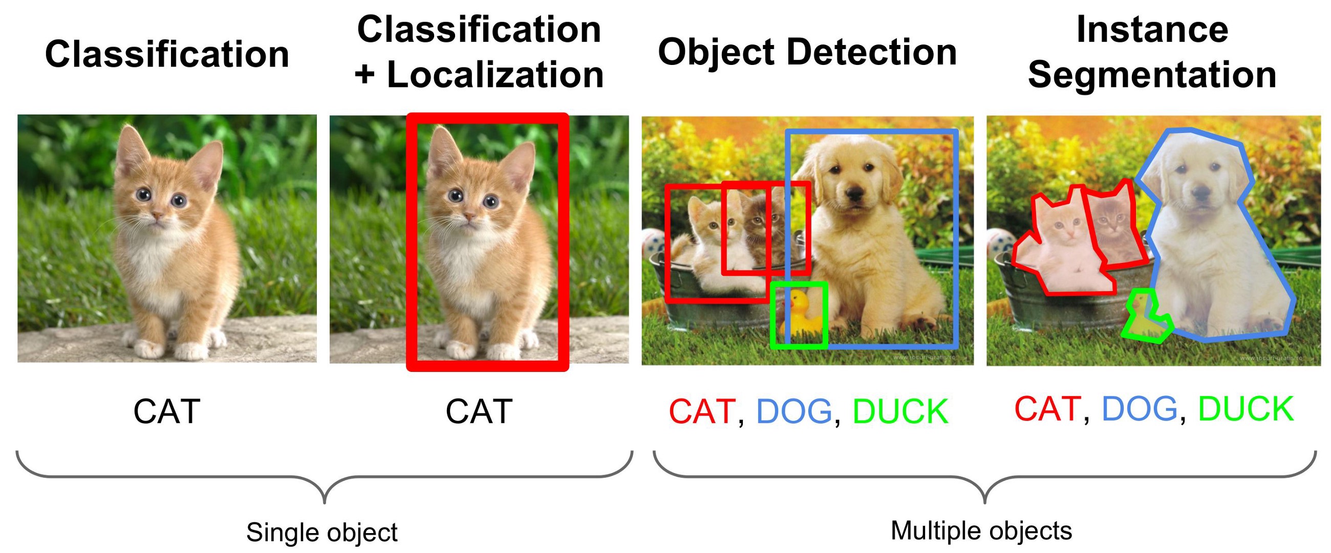
In order to be able to grasp the basic concepts of deep learning, the goal is first defined, often in the form of a question: „Does this person look cheerful?“ or „What is this word?“. These questions are usually defined in such a way that a correct result can be assigned to the input (e.g. a picture). Here it also becomes clear that the data plays an essential role—it must be clear what can be seen in the input and what the corresponding output should be. In the following you can see a small clarification. Each image displays the input for the artificial neural network. The task is named above each image.

Classification means that in the end the network should predict that you can see a cat in the image. Classification + Localization additionally wants to predict a bounding box around the cat. In Object Detection each object in the image needs to be classified and found by a bounding box. And in instance segmentation each pixel of the image will be assigned to one class—or even more complex—to one coherent object (e.g. each cat will be handled separately).

Data! We Need Data!

The processing of artificial neural networks is divided into two stages: training and validation. During the training phase the artificial neural networks get to see the same data over and over again and during the validation phase new different data are fed in to test how it performs on unseen data. There is a differentiation whether the neural network learns the training data by heart (so-called overfitting) or whether it is able to adapt to other data—to generalize.

The major challenges in this context are how to generate meaningful training and validation data, how to transform the data to be able to feed it into the network, and how to structure the input, output and architecture of the neural network.

But What is so Special About Deep Learning?

Looking at small children and their first attempts to ride a bike, you can see that they keep trying and learning from mistakes in such a way that in the end they manage to stay on the bike and jet away. However, if you have to explain to a child how to behave on their first ride on a bike, you will quickly realize that it is not that easy, because you have to define a set of rules. „Sit on it, hold on tight and kick off“? You wouldn’t get very far with such a statement. This example is also very difficult to describe mathematically or algorithmically, where the strengths of deep learning are shining. All basic actions, all emergency plans and all „what should I do if…?“—an artificial neural network learns independently without anyone having to describe exactly what it has to learn in detail.

Returning to a somewhat simpler example, given a picture we want to tell if there is a dog in it. For us humans this question is very easy to answer as we have probably seen several dogs in several poses and in several environments in our lifetimes. But what makes a dog identifiable as a dog? Its fluffyness? Its fur? Its tail? An artificial neural network learns exactly these characteristics and „layers“ them in such a way that finally a clear answer „yes“ or „no“ can be offered. If, for example, you look at a convolutional neural network, these layers can even be interpreted. If an image with a dog in the size \(100 \times 100\) pixels is assumed, a window of \(10 \times 10\) is shown to the first layer. In this case obvious information can be extracted. Where is a vertical edge? Where is a horizontal edge? Where is a diagonal edge? Such information is then shown again to the next layer in a smaller (e.g. \(5 \times 5\)) window, which can then tell what a coherent texture there is, i.e.. a grid. The information gains in significance and finally the neural net is able to tell whether a dog is present or not. A detailed illustration can be found in [3].

From here to there: Basic Concepts of Artificial Neural Networks

Fully Connected Neural Network

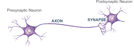
Now we’ll come to the fun part—the mathematical background. What are the components of an artificial neural network and how can they be described mathematically? As mentioned before, artificial neural networks are inspired by a human brain, so let’s start there. Basically, a human brain consists of countless neurons. These neurons are partly linked with each other by synapses. The information is transmitted via electrical impulses which cause the potential of the respective neuron to rise. If this potential exceeds a threshold, this neuron fires an electrical impulse to all subsequently connected neurons. The strength of this impulse is controlled by the synapses, which transmit („weighs“) only a part of it. The stronger this fraction is, the stronger is the synaptic connection between the two neurons and the more likely it is that both fire simultaneously. This was first recorded 1949.

Hebbian Theory: „Neurons that fire together, wire together“

On the basis of this biological point of view, the mathematical model can be formulated. First, an artificial neuron, a so-called perceptron, is constructed. This must fulfil the property that an output signal needs to be formed on the basis of the input signals it receives. This is referred as activation function, which can be any mathematical function. Finally, this means that a single perceptron weighs all its inputs by synapses, adds them up and forwards them via the activation function—this was described by Rosenberg in 1958. This single perceptron is capable of solving simple classification problems. However, at that time it was discovered that the problem of linear separability, i.e. if the problem is more complex, a perceptron could not solve an XOR problem. An XOR problem can fairly simply described by a room with two light switches. When one light switch is pressed, the light turns on. If both light switches are pressed, the light turns off again. And if no light switch is pressed, then the light stays off. However, the underlying mathematical problem cannot be solved by a single perceptron, which is why several layers of perceptrons are concatenated in the following—et voilà—we’ve formed our first neural network.

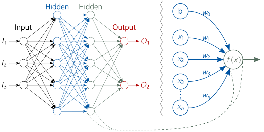
\(f_{MLP} = a^n\left(\boldsymbol{W}^n a^{n-1}\left(\boldsymbol{W}^{n-1} \cdots a^1 \left(\boldsymbol{W}^1\boldsymbol{x}+\boldsymbol{w}_0^1\right)\cdots+\boldsymbol{w}_0^{n-1}\right)+\boldsymbol{w}_0^n\right)\)

To make the point a little clearer the mathematical clarification follows. \(\boldsymbol{x}\) is the input of the neural network, for example an image. \(\boldsymbol{W}_i\) is the weight matrix (the synapses) for the current layer \(i\) with the size \(N \times M\). \(N\) is the number of neurons in the current layer and \(M\) is the number of neurons in the previous layer containing the learnable parameters \(\boldsymbol{\theta}\). \(\boldsymbol{w}_i^o\) is the weight matrix of the bias neuron, which has only connections to the current layer \(i\) and also contains \(\boldsymbol{\theta}\). \(a_i\) is the activation function of the current layer \(i\). Thus it becomes obvious that a neural network is nothing but a nesting of mathematical operations.

 

But … How does this Magic Work?

After the XOR problem has been solved in theory, the question arises how to systematically optimize all learnable parameters in a way that finally an optimum of the neural network is reached, which is „good enough“ for the actual problem. For this purpose, a so-called „loss function“ is introduced, which compares the output of the artificial neural network (\(y_{pred}\)) with the true output (\(y_{gt}\)) of the given data. This can be quite banal and achieved by simply calculating the absolute difference between \(y_{pred}\) and \(y_{gt}\). The deciding factor is that a convex difference function can be formulated which has a single minimum.

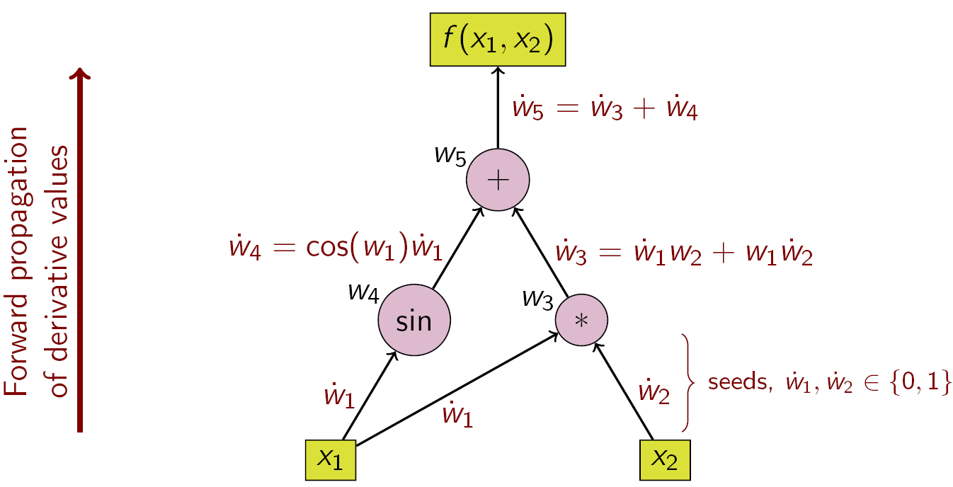
In the next step the derivation of the loss function is calculated — who can remember what the derivation of a function is good for? Right, it indicates the slope of the function! The derivative function in a vector field is called gradient and it points either in the ascending or descending direction of the multidimensional function. It has already been shown that an artificial neural network is only a nesting of mathematical operators, so it is also possible to guide the gradient back through all operators from the end to the beginning (for more information, take a look at computational graph or see Stanford CS231 Lecture).

What does this whole thing do with the gradient? The goal is that the difference between true and predicted output is as small as possible, the loss function should be minimized and the gradient should point to the minimum (this is called gradient descent). So if the gradient points in the direction of the minimum and this is passed through the complete artificial neural network (also called „backpropagation„), then it is aimed to find a state of the artificial neural network in which the loss function is smallest. More precisely, by optimizing each parameter of each operation in the artificial neural networko by backpropagating the gradient of the loss function, you can always find at least one local minimum of the loss function.

Activation Function

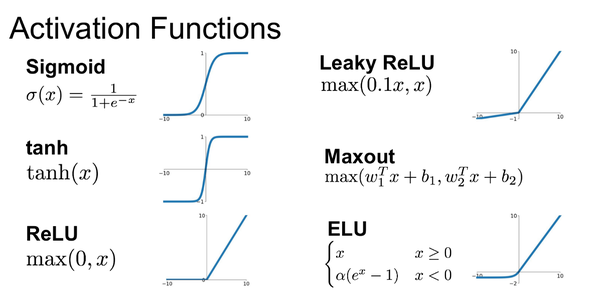
The formulation of a feed-forward artificial neural network as shown before is explained quite quickly and easily. However, you may find that it’s missing one ingredient: the activation function. An active neuron in a human brain acts according to a mathematical function that operates according to a non-linear pattern. This non-linearity plays an important role in whether a complex problem can be solved at all. If one imagines that the activation function is a linear function, the complete neural network can be represented by a scalable value. Specifically, in this case all \(a\) of the formula above would be replaced by \(1\) and finally the weight matrices can be combined into one value, so as to represent a complete neural network with one single perceptron.

One of the most popular activation functions is the Rectified Linear Unit (ReLU). In 2000 this activation function was presented for the first time by Hahnloser et al. with a biological background and mathematical foundation. In 2011, it has been shown empirically, that ReLU performs better than other non-linear activation functions, like the sigmoid or tanh functions. Mathematically, a ramp function is depicted and an analogy to the half-wave rectification in electrical engineering is obtained. For an alternating current signal only the positive or the negative half-wave is passed, completely cutting of the other half-wave. Regarding artificial neural networks, ReLUs offer a high gradient feedback, since half of the operating range is represented by a linear function, which provides constant high backpropagation of the gradient. This counteracts the vanishing gradient problem, which occurs mainly in the saturation areas of the activation function and makes the gradient too small for having an impact. In addition, depending on the initialization method of the values \theta, a regularization effect (avoiding to memorize training data) is created, since typically at least 50% of the input signal is fed into the ReLUs with negative values. There are of course several other activation functions and each one has its peculiarities, but ReLU is the best to-go tool and works in most applications.

Convolutional Neural Networks

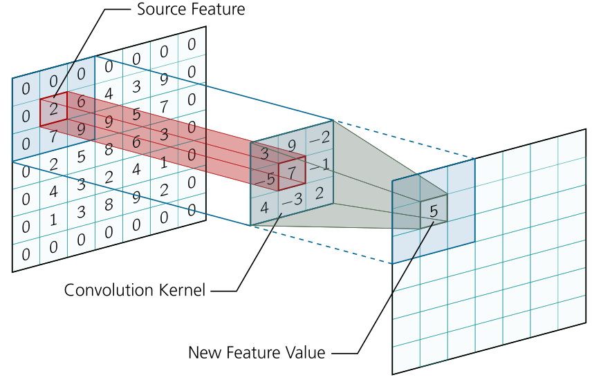
Convolutions are probably the most important concept in deep learning today. The basic idea is to create an ordered procedure that allows two different sources of information to be intertwined. The two information sources represent a high dimensional input (e.g. image) or feature maps (output of a convolution layer) and the convolution kernel, where the input/feature maps remain constant and the kernel represents the amount of intertwining. In order to perform a convolution only a small fraction of the input will be used. For this a sliding window is used. Imagine you can only see \(10 \times 10\) pixels of an image, you take them and multiply them element-wise with each element of the kernel. At the end you summarize all multiplications and get only one value. By this way you get to see only parts of the image and always calculate these snippets with the same values from the kernel. This makes it a cost-efficient method, since the kernels only see a fraction of the input and therefore use a local transformation. Repeatedly, however, the same kernels are applied globally to the image. In traditional signal processing the kernels (so-called filters) are handmade and are responsible for a particular effect. In convolutional neural networks these kernels are filled with optimizable parameters and backpropagation is applied to them. This allows the artificial neural network to learn which parameters the kernel needs to solve the problem.

An essential design choice of the CNN structure is that the input size is reduced with the network size, while increasing the number of feature maps per layer. This concept is called receptive field.

Receptive Field: The Area of the Input to the entire Artificial Neural Network the Output gets to see.

It reduces the input size while increasing the information density at the same time. The size of the input can be reduced in two ways:

The first possibility is the introduction of pooling layers. After the creation of the feature maps by convolution, the strongest feature — MaxPooling — or the average of the features — AveragePooling — is extracted at the current position of the kernel and written to the corresponding position in the new feature map. This is a computationally cheap variant without parameters that have to be learned, which only allows to pass on the only the most relevant features. A major disadvantage, however, is the loss of information, as most of the values in MaxPooling are simply discarded and the assumption that all features in AveragePooling are equivalent, while at the same time the information about the local origin is lost in both cases.

The second option is not to take each position for a snippet out of the input, but to set the next position using an overshoot factor (so-called stride). This offers the major benefit of considering all values from the feature maps so that none of the information is lost—if the stride is set correctly. Naturally, the local information can shift as a result of the convolutions and the defined stride. In detail, this means that all information within the size of the kernel patch is written to the respective location in the next feature map.

Normalization

Deep learning is called deep learning because a large number of layers (mathematical operators) are concatenated. Here the vanishing gradient problem can arise.

Vanishing Gradient Problem: The Derivation of the Gradient and its Feedback by Backpropagation gets too small from Layer to Layer.

Additionally, a so-called covariate shift can occur, which causes a bias of the training data on the weights. To avoid this, normalization techniques were introduced, which allow to force the outputs of each layer into a certain value range. For example, many network architectures use batch normalization, which empirically shows faster convergence, regularization and avoidance of covariate shift. However, this effect was only observed in models where the batch size (the number of input data per iteration) was large enough and the network architecture deep enough. In this respect, further normalization types were introduced (instance normalization, layer normalization, group normalization, weight normalization…) which normalize the values in different ways and show the standard deviation and variance of the individual input data. You can see this in the following figure.

Each cube represents a four dimensional space. \(N\) is the batch size, \(C\) is the number of feature maps, \(H\) and \(W\) are the spatial height and width. First the blue section is chosen using the normalization technique. Next the standard deviation and the mean is calculated within the blue section. Finally, each value in the blue section is recalculated in the value range by its standard deviation and mean.

Lessons learned…

First of all: Wow—you have really read everything and I thank you very much for that! In this article I wanted to show that deep learning is no witchcraft and you shouldn’t be afraid of evil artificial intelligence. Basically, I dare to say that artificial neural networks are nothing more than a solution to perform a special pattern search. I hope I also managed to bring more light into the dark and to visualize artificial neural networks and their principle of effect.

Read on

You might wanna have a look at our deep learning portfolio. If you are looking for new challenges, you might also want to consider our job offerings for Data Scientists, ML Engineers or BI Developers.

References

• [1] Medium Blog about DL4ObjectDetection
• [2] Meme with Leonardo di Caprio from the movie „Inception“
• [3] How do neural networks recognize a dog in an image?
• [4] Illustration of real neurons
• [5] Example of a computational graph
• [6] Overview of different activation functions
• [7] Influence of MaxPooling and AveragePooling
• [8] Yuxin Wu and Kaiming He. Group normalization. arXiv preprint arXiv:1803.08494, 2018.
• [9] Frank Rosenblatt. The perceptron: a probabilistic model for information storage and organization in the brain. Psychological review, 65(6):386, 1958.
• [10] Donald Hebb. 0.(1949). The organization of behavior, 1957.
• [11] Xavier Glorot, Antoine Bordes, and Yoshua Bengio. Deep sparse rectifier neural networks. In Proceedings of the fourteenth international conference on artificial intelligence and statistics, pages 315–323, 2011.
• [12] Yann LeCun, Yoshua Bengio, et al. Convolutional networks for images, speech, and time series. The handbook of brain theory and neural networks, 3361(10):1995, 1995.
• [13] Yann LeCun, Bernhard Boser, John S Denker, et al. Backpropagation applied to handwritten zip code recognition. Neural computation, 1(4):541–551, 1989.
• [14] https://deepmind.com/blog/alphazero-shedding-new-light-grand-games-chess-shogi-and-go
• [15] https://www.inovex.de/blog/deep-learning-fundamentals/
• [16] https://www.inovex.de/blog/neuroevolution/