
When you are working with highly connected datasets, you might find traditional relational databases a little cumbersome to work with. Luckily, specialized databases for all kinds of use cases are available nowadays. Time series databases store time series data, vector databases store vector spaces, and graph databases store highly connected datasets that are best conceptualized as a graph.
In this article, we give an introduction to graphs and graph databases and discuss some example data science use cases. We also look more closely into graph query languages, the primary tool for interacting with graph data, by comparing the two major languages Gremlin and Cypher.
Graph Databases: A Gentle Introduction
With how connected the real world is, it is no surprise that the data sets that emerge in real-world use cases are a lot more connected than they used to be:
- Social networks connect users as friends or colleagues (or friends of friends and so on).
- Users of a media platform connect pieces of content by consuming them.
- In the financial sector, graphs emerge as people, banks, and businesses have financial transactions with one another.
The question is, how do we represent and store these datasets in a way that allows us to analyze these connections explicitly and see our data points as what they really are: nodes in a network of connections.
What are graphs?
As is often the case, mathematics comes to the rescue and provides a very established and well-understood concept for representing connected elements: graphs.
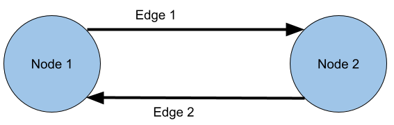
Mathematically speaking, a graph consists of two sets: A set of nodes (entities or items we are interested in) and a set of pairs, called edges, that connect two nodes. Mathematicians distinguish between directed and undirected graphs, but for our purposes, we only look at directed graphs, where each edge has a direction. A simple example could look like this.
Based on this simple concept, mathematicians and computer scientists have developed countless algorithms for working with graphs. To name only a few, graphs can be searched by traversing edges, tightly connected clusters of nodes can be identified, and nodes can be ranked based on their centrality in the graph.
Graph databases are based on exactly this mathematical concept. You store your data not as rows in tables, but directly as nodes and edges. Typically, nodes and edges are labeled, so that different kinds of entities and relationships can be distinguished. Each node and edge can also hold additional information in the form of properties.

This is then called a property graph. Nodes are the entities you are interested in, and all information about them and the relationships between them are stored in properties.
Where can you store your graph data?
Several different graph database products exist for storing and then working with property graphs. For example, Amazon offers the fully managed AWS Neptune. It supports several different ways of interacting with your graph through graph query languages.
Neo4j is an independent graph database you can host and maintain yourself. Ready-made Docker containers are available for getting up to speed very fast. In addition, a fully managed cloud version is available as Neo4j AuraDB.
It is worth noting that there is another kind of graph you can use to store your data: RDF graphs. RDF (Resource Description Framework) and the corresponding query and processing language SPARQL come from the world of semantic modeling and are most useful for what are called knowledge graphs. AWS Neptune actually supports RDF graphs in addition to property graphs.
What are the advantages of graph databases?
In cases where you deal with datasets that are highly connected, especially if you are explicitly interested in these connections between your data points rather than just the data points themself, graph databases provide some exciting benefits over traditional relational databases:
- Explicitly build the graph you are thinking about. If you naturally start to conceptualize your data as a graph and draw up example cases on a whiteboard, it is a lot easier and faster to directly translate your ideas for analyzing your data into queries in a query language designed for graphs, rather than having to shift perspective into a relational data model.
- Flexibility. Because of the relative simplicity of graph data models (nodes connected by edges), your data model can change dynamically with your use case. Nodes can be added or removed, relationships can be redirected or re-labeled, and properties of both nodes and edges can be changed.
- Ready for complex ML use cases. Because graph databases explicitly represent and store not only individual data points but also the various connections between them, machine learning algorithms can take these connections into account and see each data point in context to the entire dataset. One particularly interesting tool are graph embeddings that represent each node (or entire sub-graphs) as vectors that can be fed into ML algorithms.
Typical Use Cases for Graph Databases
As briefly mentioned above, any dataset that contains interesting or important connections between data points can benefit from graph databases. One interesting application is recommender systems, which we discussed in more detail here. Let us look at some more concrete examples and what the data model in these use cases might look like.
Social networks
For a social network platform connections between people are essential, so storing user data in nodes and representing friendship relations as edges makes intuitive sense.

The idea of finding central nodes in a graph mentioned above actually originated in the context of social networks. There are several different definitions of centrality, useful when trying to find the most influential person in a group. The same algorithms have since been used in other contexts, like finding key infrastructure nodes in the Internet or urban networks (roads, power, and water networks).
User Journey Graphs
For companies that provide access to digital media like movies or music, interesting connections between these pieces of content can emerge from users consuming them.
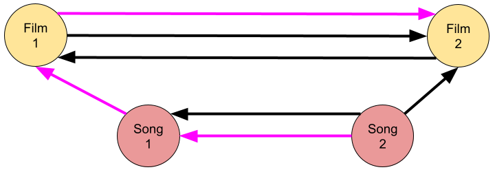
The data model above allows us to directly use graph algorithms for finding pieces of content that are central to a certain portion of our user base, providing interesting insights for recommendation systems. We can also find interesting connections between different pieces of content by looking for unexpected connections through users that consumed both pieces of content.
The connections themself also reveal interesting patterns in user behavior. If we follow the edges of individual users, we can analyze the journey this user has taken through our content.
Fraud Detection
Finally, credit card institutes use graph technology for automated fraud and anomaly detection. A simplified data model for this use case might look something like this.
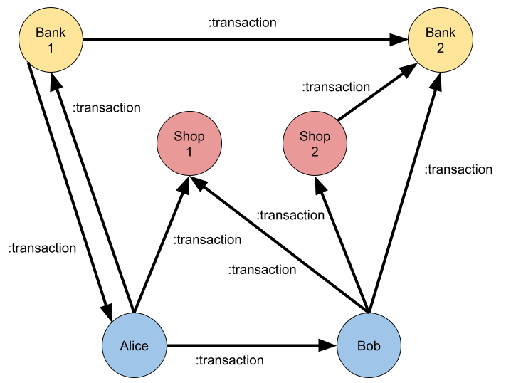
Several graph algorithms are perfectly suited for finding anomalies or potentially fraudulent transactions in a graph like this. Community detection algorithms for finding Weakly Connected Components or the Louvain algorithm can find fraud rings consisting of businesses and people laundering money. Additionally, similarity algorithms like KNN can be used to find potential fraudsters based on their similarity to known fraudsters.
Graph Query Languages: Comparing Gremlin and Cypher
Once your data is modeled as a property graph and stored in a dedicated graph database, you need to interact with your data for analysis. That’s where graph query languages come in. Here we demonstrate and compare two very different query languages called Gremlin and Cypher.
To compare the two approaches to querying graph data, we look at the following graph from an example provided by Neo4j here.
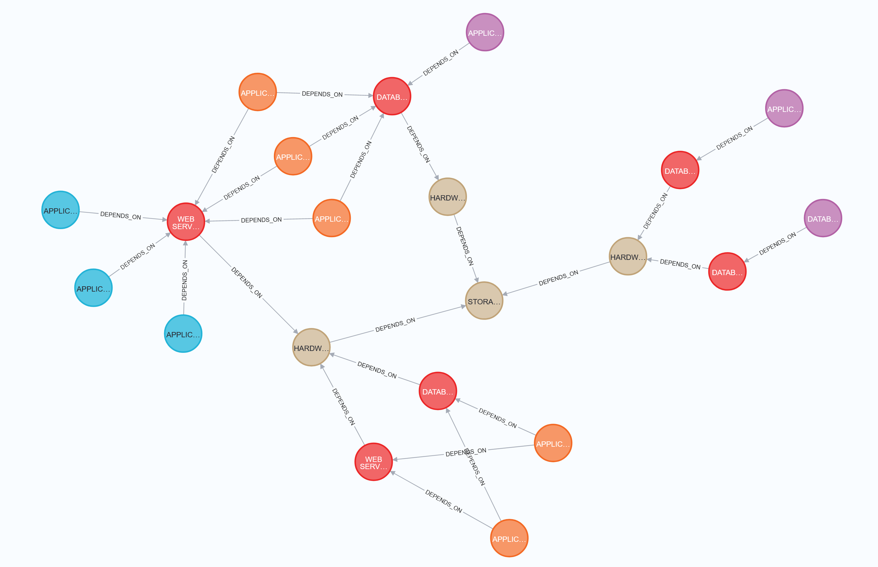
The graph contains network components, connected by dependency edges. Every network component has properties like hostname, IP, and type. The nodes in the image above are labeled with their type. For the questions we are going to answer, four kinds of nodes are of particular interest:
- The blue application nodes represent internal (Intranet) web pages.
- The orange application nodes represent public (Internet) web pages.
- The brown nodes are hardware components.
- The red nodes are virtual machines, which always depend on some hardware component.
For the graph above, we want to answer the following basic questions:
- Which internet pages depend on the virtual machine with the hostname WEBSERVER-1?
- Which hardware resources does each intranet page ultimately depend on, i.e. what is the hardware resource at the end of each dependency chain starting at an intranet page?
- How many resources of each kind are in the Network, and what are their hostnames?
Gremlin
Gremlin is part of the Apache TinkerPop graph computing framework. Queries written in Gremlin are essentially algorithms composed of traversal steps. The main effect of these traversal steps is to traverse the graph, following edges from node to node either forward or backward. Along the way, you’ll make use of steps with side effects. These side effects include saving graph elements in local variables, grouping elements by property values, or aggregating property values. We will see several of these while answering the questions from the previous section.
Question 1
The basic traversal steps we’ll use in these examples are in() and out(). Starting from a node, they follow in- or our-edges respectively to get to the next node. But other traversal steps to explicitly move to edges themselves to work with their properties exist in Gremlin. To start your traversal, you can use either the V() or E() step. They return all vertices (nodes) or all edges in the graph, respectively. from there you can use has() to narrow down the starting points for your traversal.
For the first question, we can start from the node with the hostname WEBSERVER-1, follow all incoming edges backward, and from these nodes filter out all nodes that do not have the Internet label.
|
1 2 3 4 5 |
gremlin> g.V().has('host','WEBSERVER-1').in().hasLabel('Internet').valueMap('host','ip') ==>[ip:[10.10.35.2],host:[support.acme.com]] ==>[ip:[10.10.35.3],host:[shop.acme.com]] ==>[ip:[10.10.35.1],host:[global.acme.com]] |
The results of our gremlin queries are typically dictionaries that map the desired property names to their values. Since we have three internet nodes dependent on WEBSERVER-1, we get three result dictionaries.
Question 2
The second question requires us to follow a path until a certain condition is met. This can be accomplished using the .repeat().until() construct. We start again by finding our starting node, in this case, all nodes labeled with Intranet. Here we can use .as() to store the results of this step in a variable, so we can access them later to extract the host and ip properties. We then specify which steps should be repeated from each starting node which in this case is a simple out step, following outgoing edges. We do this until we reach a node where the outE traversal step, usually returning outgoing edges, returns false.
The project step then specifies the values we want to display as our result. This is then followed by an equal number of by-modulators. The by-modulator specifies which values should be used for the preceding step. In the case of the project step with four keys, we supply four by-modulators. The first two modulators access the properties host and ip from the previously stored starting nodes. Since after the repeat().until() steps the current location in the graph is the final hardware node we are interested in, we can simply access its properties host and ip in the other two modulators.
|
1 2 3 4 5 6 7 8 9 10 11 |
gremlin> g.V().hasLabel('Intranet').as('intranet') .repeat(out()).until(__.not(outE())) .project('i_host','i_ip','h_host','h_ip') .by(select('intranet').values('host')) .by(select('intranet').values('ip')) .by('host') .by('ip') ==>[intranet_host:events.acme.com,intranet_ip:10.10.35.2,hardware_host:SAN,hardware_ip:10.10.35.14] ==>[intranet_host:intranet.acme.com,intranet_ip:10.10.35.3,hardware_host:SAN,hardware_ip:10.10.35.14] ==>[intranet_host:humanresources.acme.com,intranet_ip:10.10.35.4,hardware_host:SAN,hardware_ip:10.10.35.14] |
Question 3
The third question requires some grouping and aggregating, which works a little differently than you might be used to from declarative languages like SQL. Grouping is achieved by the group() step, which expects two by modulators. The first tells the group step which property should be used for grouping, while the second tells the group step which value needs to be produced for each group.
Since we want to produce two values per group to answer the third question (the number of nodes per group and a list with all host names), we use the fold() step to wrap all elements within a group, so that we can use match() to perform multiple queries on them. The first subquery counts all elements within the folded group, while the second subquery first unfolds the group in order to access the host value from each node and fold them into a new list. Finally, we can select the values produced by the two subqueries.
|
1 2 3 4 5 6 7 8 9 10 11 |
gremlin> g.V().group().by('type').by( fold().match(__.as('x').count(local).as('count'), __.as('x').unfold().values('host').fold().as('names') ).select('count','names')) ==>[DATABASE SERVER:[count:4,names:[CUSTOMER-DB-1,CUSTOMER-DB-2,ERP-DB,DW-DATABASE]], STORAGE AREA NETWORK:[count:1,names:[SAN]], DATABASE:[count:1,names:[DATA-WAREHOUSE]], APPLICATION:[count:10,names:[CRM-APPLICATION,partners.acme.com,ERP-APPLICATION,events.acme.com,intranet.acme.com,global.acme.com,humanresources.acme.com,support.acme.com,shop.acme.com,training.acme.com]], HARDWARE SERVER:[count:3,names:[HARDWARE-SERVER-1,HARDWARE-SERVER-2,HARDWARE-SERVER-3]], WEB SERVER:[count:2,names:[WEBSERVER-1,WEBSERVER-2]]] |
The result is then a nested dictionary, mapping a dictionary with the count and hostname list to each group key.
Cypher
Cypher is very different from Gremlin, in that it is a purely descriptive query language, while Gremlin is imperative. It was developed for Neo4j, which is one of the most popular graph databases on offer. The core of the language was since open-sourced as openCypher and it’s now supported by several other graph databases.
Cypher queries work by matching patterns in the graph topology, filtering and joining the matched nodes and edges, and finally returning the required properties from the result.
Question 1
We use the most basic clauses of Cypher to answer the first question. We MATCH all pairs of nodes that are labeled with Internet and VirtualMachine that are connected by an edge. In order to filter the matched parts of the graph, we use the WHERE clause to only keep virtual machines with the required hostname. From the internet nodes in the result set, we can then RETURN the properties host and IP.
|
1 2 3 4 |
MATCH (inet:Internet)-[:DEPENDS_ON]->(vm:VirtualMachine) WHERE vm.host = 'WEBSERVER-1' RETURN inet.host as host, inet.ip as ip_address |
Result:
| host | ip |
|---|---|
| shop.acme.com | 10.10.35.3 |
| support.acme.com | 10.10.35.2 |
| global.acme.com | 10.10.35.1 |
Question 2
In addition to matching individual edges, Cypher also lets you describe paths of variable length. The modifier *1.. in our edge description specifies that we are looking for a path of any length from an Intranet node to a Hardware node. After the first MATCH clause, the result still contains extra paths, because each of the three intranet nodes depends on two hardware nodes along the same path. We can filter out the paths to all intermediate dependencies by describing another pattern that we do not want to see at a hardware node, namely that the final node should not have any further dependencies. The WITH clause allows us to define local variables. Here we access the first and last node of each path after the filter, so we can more easily extract the properties host and ip in the RETURN clause.
|
1 2 3 4 5 6 7 8 |
MATCH p=(intranet:Intranet)-[:DEPENDS_ON*1..]->(hardware:Hardware) WHERE NOT (hardware)-[:DEPENDS_ON]->() WITH NODES(p)[0] as intranet_node, LAST(NODES(p)) as hardware_node RETURN intranet_node.host as intranet_host, intranet_node.ip as intranet_ip, hardware_node.host as hardware_host, hardware_node.ip as hardware_ip |
Result:
| intranet_host | intranet_ip | hardware_host | hardware_ip |
|---|---|---|---|
| events.acme.net | 10.10.35.2 | SAN | 10.10.35.14 |
| intranet.acme.net | 10.10.35.3 | SAN | 10.10.35.14 |
| humanresources.acme.net | 10.10.35.4 | SAN | 10.10.35.14 |
Question 3
For the last question, we can use some of the built-in aggregation functions. We first match all nodes in the graph. When using aggregations in Cypher, every property that is mentioned but not aggregated before the aggregations is implicitly used as a grouping key. Here we group by the type property of the matched nodes, count them, and collect the host names of all nodes.
|
1 2 3 4 |
MATCH (n) RETURN n.type as type, count(*) as count, collect(n.host) as names |
Result:
| type | count | names |
|---|---|---|
| APPLICATION | 10 | ["CRM-APPLICATION", "ERP-APPLICATION", "global.acme.com", "support.acme.com", "shop.acme.com", "training.acme.com", "partners.acme.com", "events.acme.net", "intranet.acme.net", "humanresources.acme.net"] |
| DATABASE | 1 | ["DATA-WAREHOUSE"] |
| WEB SERVER | 2 | ["WEBSERVER-1", "WEBSERVER-2"] |
| DATABASE SERVER | 4 | ["CUSTOMER-DB-1", "CUSTOMER-DB-2", "ERP-DB", "DW-DATABASE"] |
| HARDWARE SERVER | 3 | ["HARDWARE-SERVER-1", "HARDWARE-SERVER-2", "HARDWARE-SERVER-3"] |
| STORAGE AREA NETWORK | 1 | ["SAN"] |
Which Graph Query Language is Best for You?
Gremlin and Cypher take very different approaches to working with graph data and considering that one is imperative while the other is declarative, it seems like they serve two different crowds.
Gremlin is probably easier to learn for developers with a lot of experience in imperative programming languages. Just like each command in a programming language, each step in Gremlin has a clear effect. Figuring out how these effects work together to traverse a graph and produce an output is akin to writing algorithms over complex data structures.
Cypher feels more like SQL. You describe the result you want to see and the query engine finds a way to extract the required information from your graph. This is probably easier for data scientists and analysts, that are familiar with this approach to working with data.
Your choice might also depend on the graph database you are using. Since Cypher has only recently been adopted by other graph database products like AWS Neptune, some features of the language are not yet fully supported everywhere. And because it is a new offering, some query optimizations you would find in Neo4j, might not happen in AWS Neptune, resulting in generally better performance for Gremlin queries.
Conclusions
Graph-based approaches allow you to see your data in an entirely new way. Modeling several disconnected datasets in a single graph structure enables you to explore all the connections between the data points.
The basic idea of nodes connected by edges is very versatile and supports many different use cases. This allows you to use a vast range of graph-based algorithms and machine-learning approaches for analyzing your data.
Modern graph databases like Neo4j or AWS Neptune allow you to intuitively query and explore your graph data using graph query languages like Gremlin or Cypher. They also often come with graph algorithms and machine-learning ready to use, so you can get up to speed with your graph in no time.


