Digitize your Receipts using Computer Vision

“Would you like the receipt?“—It’s hard to say no to that. Not because you actually want it (you may even throw it in the trash before exiting the store), but because doing otherwise might hurt the feelings of the cashier. But if you take a closer look, you will discover that a receipt carries all kinds of wonderful information. The most obvious data point is the total amount, which is useful in tracking your monthly expenses. Close to that you’ll typically find a list of individual items. This you could use to inform your flatmate or spouse that you already bought the milk (but forgot the toilet paper) they wanted to pick up after work. The date of purchase might be useful if you need to decide if the eggs in the fridge are still safe to eat. Tracking receipts over a longer period of time might reveal trends in item prices and maybe even tell stories about your life, like that time you decided to eat more healthy food.

Alas, all these use-cases require the information to be digital instead of being printed on thermal paper! Until retail decides to start using digital receipts, that means that you’ll have to manually type the information into a computer—and we can probably agree that while you may record some of that information (like the total amount), transcribing all of it is simply not realistic. But isn’t this the age of automation where anything is possible? If we can put self-driving cars into space, we can surely digitize the information on a receipt, can’t we? Well yes, we can. Google Lens, Evernote, Expensify, PaperScan and taggun.io are just some of the many apps and services you could use. So problem solved, right? OK, thanks, bye!

But wait! Don’t you want to know how these apps do it? Then you have come to the right place, because in the following I will describe our take on recreating the basic functions of the aforementioned apps, show the engineering involved in tackling this task, describe what did not work the way we thought and why that may have been the case. And yes, there will be code so you can try it out for yourself!

Besides, receipt digitization is actually a great example for computer vision in general, where the goal is to extract information from raw pixels. The approaches and techniques outlined here can certainly be modified to cater to other use-cases as well. And believe it or not: receipt understanding is actually an active area of research—take a look at this 2017 paper by Raoui-Outach et al. or the ICDAR 2019 Robust Reading Challenge.

System Overview: What Will It Do?

Given a picture of a receipt, perhaps taken with your smartphone, this is what we want to achieve:

1. Find the receipt in the image,
2. Enhance the image by cropping the receipt, correcting for perspective distortion and increasing text contrast.
3. Extract the text in machine-readable form, i.e., do optical character recognition.

To keep this post somewhat contained, we will ignore all the steps that come before and after. In particular, we will not cover how to actually take the picture, nor will we discuss what to do with the information once it is extracted. We will also assume that the pictures are of reasonable quality and resolution, that a receipt is present and covers most of the picture.

This leaves us with these three steps: First, detect the receipt; second, extract the receipt and improve contrast; third, extract the text:

As promised, we will describe the details of each step in the following. But first:

Step 0: Aquire Some Data

Before we can start extracting text, we need something to extract it from. A quick search reveals that there are indeed some datasets we could use. However, none seem to fit our goal just right. For example, ExpressExpense’s Massive Receipt Archive has many images of receipts, but overall resolution is quite low, the receipts are not always fully contained in the image, and there is a watermark at the bottom of each image. Jens Walter’s receipts, on the other hand, are very high quality scans, but are already cropped so that the image contains nothing but the receipt.

So we decided to collect our own data instead. This way, we could ensure the quality as well as the difficulty of the images. We collected 68 images in total, where 9, 11, 7, 10 and 12 receipts were from the German grocery chains Aldi, Edeka, Lidl, Rewe and Scheck-In, respectively. The remaining 19 receipts were all from different stores. For good measure, we also threw in a public transport ticket, because: why not?

We made sure that the background was not too busy and that the contrast between it and the receipt was high. All receipts were oriented more or less upright without too much perspective distortion to not make our lives harder than necessary. However, most of the receipts were crumpled during transport so that they had folds and creases and some had washed out letters as well to make the task not too easy after all. Below you can see some examples of the images we collected:

Step 1: Detect the Receipt

The goal in this step is to detect the areas of the image that show the receipt. Since a receipt in general is a rectangular piece of paper, it makes sense to describe that region using a quadrilateral, i.e., a polygon of four vertices \(\{\mathbf p_1, \mathbf p_2, \mathbf p_3, \mathbf p_4\}\). The vertices should be chosen such that the polygon covers as much of the receipt and as little of the background as possible. A picture is worth a thousand words, so here is an example of what we want:

Surprisingly, this turned out to be the most complicated part of the whole project. The process can again be broken down into three parts: image preprocessing, receipt detection, and finally estimating the corners of the polygon. Let’s start at the beginning.

Step 1.1: Image Preprocessing

Though color may provide useful information to discriminate fore- and background, we found that the contrast between mostly white and smooth receipt and mostly non-white, generally non-smooth background was large enough to separate the two. Thus, we converted the images to grayscale, which conveniently reduces the data by two thirds and speeds up the subsequent processing. This is common in many computer vision applications, as texture often (but not always) carries more relevant information than color¹, and including color is essentially a source of noise that machine learning could overfit on.

We also normalized the global illumination by removing slow illumination gradients using an old image processing trick: Slow gradients correspond to low frequency modulation of the image intensity, thus filtering the image with a high-pass filter should even out the global illumination. This high-pass filter can efficiently be implemented using the discrete cosine transform (DCT): Transform the image into frequency space, zero out the low frequency components, and transform the image back into the spatial domain. Note that we use the DCT instead of the discrete Fourier transform (DFT) to avoid dealing with complex numbers which inevitably arise when zeroing out the low frequency DFT components. Since the whole process changes the magnitude of all pixels, we finally normalize the pixels to the range [0:1]. The result of the preprocessing can be seen here:

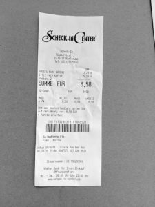
With the help of both scipy and scikit-image, we can accomplish the above in just a few lines of Python:

Step 1.2: Receipt Detection

Given the preprocessed images, the next step is to segment the image into pixels that show the receipt and those that do not. We tried several different methods ranging from automatic thresholding according to Otsu to Superpixel Segmentation. In the end, however, it turned out that a simple global threshold followed by some binary morphology and blob detection worked just fine. More specifically, we blur the image to suppress noise and apply a threshold at 60% intensity to get an initial segmentation. From there, we apply binary closing to remove small false detections in the background and fill defects along the contour. Hole-filling closes the holes caused by larger texts, logos and bar codes on the receipt. Finally, we discard all but the largest blob in the image:

Again, scipy and scikit-image make all this very easy:

Note: This approach will inevitably fail if the background has a similar brightness as the receipt. In this case, you could compute the edge image using gradient operators, the Canny or Deriche edge detectors, or some other algorithm. Regardless of the method, you will need to filter out edges detected in the background and on the receipt (e.g., from text and creases), which is non-trivial and the reason we chose the simple method above instead.

Step 1.3: Corner Detection

At this stage you might think that you could simply place the polygon vertices in the corners of the outline. Indeed, this was the first thing we tried and while this works here, in the general case it will not. Consider the rightmost receipt (from “Aldi“) of the examples presented above: Here, putting the vertices in the corners would make the polygon clip the area on the left of the receipt. Additionally, the lower left corner has a very obtuse angle, which gives a hint that reliable corner detection may not be as easy as measuring the internal angles. In other cases, the receipt may be damaged, have rounded corners or even corners in weird places caused by an uneven tear.

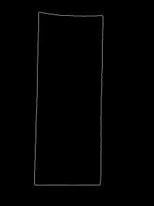
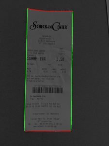
For a more robust approach, we instead focus on the edges of the receipt. Specifically, we compute the outlines of the receipt from the foreground mask (again using binary morphology) and then apply a probabilistic Hough transform to get the start and end points of the line segments in the image:

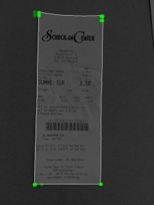
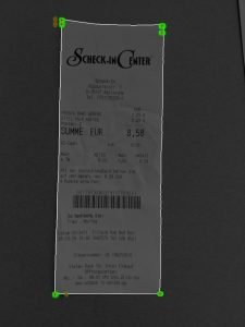
As you can see in the image and the code above, we also sorted the segments into horizontal and vertical segments. Then, we compute the intersection of each pair of horizontal and vertical segments (green blobs) to get a list of corner candidates, which we reduce to more a reasonable number with mean shift (red crosses):

This is necessary to avoid the combinatorial explosion in the next step, where we construct a polygon candidate from every possible combination of four points, e.g.:

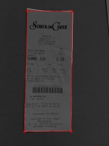
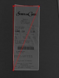
In this example, there are 10 corner candidates which result in 131 possible polygons². To determine the best of those, we find the candidate that has the highest agreement with the segments found by the Hough transform. Here, agreement is measured by the distance of the segments found by the Hough transform to the edges of the polygon. In the ongoing example, this is the candidate with the highest agreement:

Quite a good fit, don’t you think? The code to compute agreement is a little more involved than the code for the other steps, which is why we don’t show it here. It really boils down to high-school math though, so you will have no trouble figuring it out for yourself. Doing so might also be a good opportunity to try other ways to measure agreement, e.g., by computing the overlap of the polygon and the foreground mask or by rating the area and internal angles of the candidate.

What Didn’t Work?

Of course, all of the above did not just work out of the box. We tried several different approaches to detect the receipts, each with different levels of success. Here is a selection of those that failed:

Corner Detection

Our first impulse was to use a standard corner detector to, well, detect the corners of the receipt. As described above, the corners of the receipt are not necessarily the corners of the polygon we care about, so this is set up to fail. However, classic corner detection failed one step sooner, since it yielded way too many corner candidates both in the background and on the receipt. Filtering out the correct ones using SIFT and related descriptors did not work as intended.

Active Contours

Another standard approach for contour fitting goes back to Kass, Witkin and Terzopoulos: Active Contour Models, also known as Snakes. The math may look somewhat daunting, but the underlying idea is quite appealing: Forces push the contour towards nearby edges and other interesting features in the image, while, at the same time, the contour tries to resist deformation. Picture an active contour as a balloon inside a container: When filled with air, it will expand and eventually stop expanding at the boundaries of that container. Snakes can also be contracting, like a balloon that wraps around an object inside it once you let out the air. As the method is quite mature, there are many implementations available, like the one found in scikit-image.

The main issue, like so often, was finding a good initialization: When the initial contour was put inside the receipt, it would often snap onto the text instead of the outlines of the receipt. When put outside, the snake would often get stuck on other edges in the background. Additionally, the algorithm is much, much slower than the simple method outlined above.

Black-box Optimization

Inspired by Snakes, we figured it might be worth a shot to cast polygon fitting as an optimization problem and let scipy.optimize figure out the details. Ideas ranged from measuring the amount of bright pixels inside the polygon in relation to the whole image over comparing the color distribution with a distribution “learned“ from the receipts to computing the distance of the polygon boundary to edges in the image. But no matter how much we wanted this to work, in the end the optimization always got stuck in local minima far from the desired one, if it converged at all.

Deep Learning

Finally, you can’t really get away without giving deep learning a shot. The idea would be to train a CNN to directly map images to the coordinates of the polygon vertices. Such approaches have been proven to work with facial feature detection (e.g. here, here and here), so why wouldn’t it in our case? The relatively small number of training data could easily be increased using simple image transformations—Keras has a nice API for that—so we gave it a shot.

Long story short: it did not work. Regardless of network topology, loss function and optimizer, the network eventually settled for a mean shape that is close to the training data, or collapsed into a single point. With enough time (and more training data), you could probably find a solution that works, but the problem itself is somewhat ill-posed to begin with: Good locations for the polygon vertices often lie outside of the receipt and the receipt itself does not give many clues where the network should put the polygon. At the same time, there are many sources of visual noise, like text, creases and folds or geometric and perspective distortions. A stage-wise approach like the one by Sun, Wang and Tang will likely fail for similar reasons.

A much better application for a CNN might be to provide the initial segmentation, e.g., with Mask R-CNN or U-net, and then find the polygon coordinates using the method shown in step 1.3. Alternatively, you could directly learn a transformation map to rectify the receipt like Ma et al. do with DocUNet. Unfortunately the authors did not release code for training data generation nor the trained model.

Step 2: Cropping, De-skewing and Contrast Enhancement

Once the receipt is found, the next steps are to extract it from the image and boost the contrast of what’s printed on the receipt. The former means we need to both crop and de-skew the image. Both are standard operations in image processing and scikit-image provides transform.warp() to do them in one pass using a mapping between input pixel and output pixel locations. For efficiency reasons, scikit-image actually needs the inverse mapping, i.e., the mapping that, given an output pixel, returns the corresponding location in the input image. Fortunately, scikit-image also provides methods to estimate such mappings from pairs of coordinates like—you guessed it—the corners of a polygon. All we need to do is to pick a mapping and define the desired output shape for a given polygon.

As the distortion is mostly due to perspective (which maps a rectangle to a quadrilateral), it makes sense to use transform.ProjectiveTransfom. For the output shape, we simply compute the edge-lengths of the quadrilateral and construct a rectangle with width and height equal to the maximum length of the top and bottom and left and right segments, respectively. This works reasonably well as long as the receipt and camera plane are close to parallel.

With the assumption that coordinates contains the polygon vertices in clockwise order starting from the upper left corner, the code to extract the receipt is:

And here is what that does to our example:

In theory, we could stop here, but there is still some visual noise we want to get rid of in order to make subsequent optical character recognition easier. In particular, we want to remove the parts of the background that are still visible and, more importantly, the shadows and highlights caused by folds and creases. The problem might be a good fit for Gandelsman, Shocher and Irani’s Double-DIP, but then again, good old thresholding will likely also do the trick. Instead of a global threshold, though, this time we computed adaptive local thresholds according to Sauvola’s method. This method is specifically designed for OCR and works by computing a different threshold for each pixel depending on the gray value distribution around that pixel.

Formally, the threshold \(\tau(u,v)\) at the position \((u,v)\) is defined as

\(\displaystyle \tau(u, v) := \left(1 + k\,\left(2\,s_{A(u, v)} – 1\right)\right) m_{A(u, v)}\),

where \(m_{A(u,v)}\) and \(s_{A(u,v)}\) denote the mean and standard deviation of gray values in the image patch \(A(u,v)\) around the pixel at \((u,v)\). The parameter \(k\) balances the contribution of the standard deviation on the threshold and can be interpreted as some prior knowledge about the noise-level of the image. In our experiments, a square patch of \(55\times 55\) pixels and \(k=0.1\) yielded good results. Below you can see the threshold gray levels and resulting image mask, where in the rightmost image we also removed all blobs that touched the image border:

As you can see the threshold successfully suppresses most of the illumination differences while keeping the text intact. However, some characters, especially the small ones, are hard to make out in the binary image. Therefore, we first feather out the mask by Gaussian blurring and multiply it with the original (receipt) image. This effectively removes all masked regions, but with soft instead of hard edges. Finally, we increase contrast using gamma “correction“:

All this is done in less than 10 lines of Python:

What Didn’t Work?

We tried to estimate a global threshold from the gray value distribution, e.g., at the 8th percentile. While this worked in many cases, it failed when creases on the receipt resulted in strong illumination differences, like in the rightmost image at the top of this post.

We also experimented with gradient operators. The intuition was that these essentially act as high-pass filters, which would suppress the low-frequency illumination changes, but retain the high frequency details of the characters. Unfortunately, gradient operators also remove the inside of characters. We tried to counteract this with morphological closing and hole-filling, but this would also close holes we wanted to keep (e.g., the one in an O) and fuse characters that should remain separate.

Finally, we experimented with different local thresholding methods. All these methods effectively boil down to computing some statistic over the local neighborhood of the pixel of interest, such as the mean, median or z-score. However, Sauvola’s method proved to be the most robust.

Step 3: Information Extraction

This is all well and good, but in the end we still only have a bunch of pixels. To do anything more useful downstream, like tracking expenditures, monitoring your pantry and telling stories, you’ll need the text. With all that has been done so far, we could certainly go the extra mile and roll our own OCR by training a classifier to recognize individual characters like Florian described here. However, OCR requires more than that (most notably: page segmentation) and this post is already too long to open that can of worms.

Fortunately there are very good commercial and free OCR libraries out there. The most popular free option seems to be the Tesseract OCR engine, but OCRopus might also be a good option, especially if you want to explore the inner workings of OCR. Here, we use pytesseract, which is a simple wrapper around Tesseract.

Using pytesseract is simple: call image_to_string() to convert the image into a single formatted string. Call image_to_data() to get individual text fragments with recognition confidence and other useful information. For best results, make sure to use a model for your target language³:

Source image

Extracted text

Semecn-nCHrer‘ Scheck-In Rüppurrerstr, 1 D-76137 Karlsruhe Tel. 0721/35258-0 E FROSTA BAMI GORENG 3,29 ETTLI FAIR KAFFEE 5,29 A Posten: 2 - . SUMME EUR 8,58 EC-Cash EUR 8,58 MuSt \ WETTO MwSt UMSATZ AM 8.02 0,56 8,58 Mit der DeutschlandCard hätten Sie auf den Umsatz von: 8,58 EUR 4 Punkte erhalten! 175732803191070095; OE A HG Es bediente Sie: Frau . Morina Datum Uhrzeit Filiale Pos Bed Bon 28.03.19 19:48 0047573 107 028 9521 Steuernummer:; DE 188293910 Vielen Dank für Ihren Einkauf Öffnungszeiten: - Sa.: 08:00 Uhr bis 22:00 Uhr www scheck- In-center ‚de 1 2 3 4 5 6 7 8 9 10 11 12 13 14 15 16 17 18 19 20 21 22 23 24 25 26 27 28 29 30 31 32 33 34 35 36 37 38 39 40 41 42 43 44 45 46 47 48 49 50 51 52 53 Semecn-nCHrer‘   Scheck-In   Rüppurrerstr, 1   D-76137 Karlsruhe   Tel. 0721/35258-0   E   FROSTA BAMI GORENG 3,29   ETTLI FAIR KAFFEE 5,29 A   Posten: 2 - .   SUMME EUR 8,58   EC-Cash EUR 8,58   MuSt \ WETTO MwSt UMSATZ   AM 8.02 0,56 8,58   Mit der DeutschlandCard hätten Sie   auf den Umsatz von: 8,58 EUR   4 Punkte erhalten!   175732803191070095;   OE A HG   Es bediente Sie:   Frau . Morina   Datum Uhrzeit Filiale Pos Bed Bon   28.03.19 19:48 0047573 107 028 9521   Steuernummer:; DE 188293910   Vielen Dank für Ihren Einkauf   Öffnungszeiten:   - Sa.: 08:00 Uhr bis 22:00 Uhr   www scheck- In-center ‚de

While certainly not perfect, this looks pretty good: all of the relevant information is there for your taking. To improve the result, we can filter out the low confidence detections and those that are obviously too small to be text. As mentioned above, image_to_data() provides the information to do so. The default output is in a TSV (tab separated values) format, but pytesseract can automatically parse this into a python dict or a pandas Dataframe, which we’ll use here:

This gets rid of the obvious mistakes like Semecn-nCHrer‘ and the false detections caused by creases left over from the preprocessing steps. Another good way to increase recognition performance is to increase the image resolution, but be aware that this will increase the time spent in preprocessing and can also reduce the overall recognition performance. This post by “Willus Dotkom“ suggests that the optimal character height might be around 30 pixels. The tesseract wiki further suggests to add words and patterns typically found on receipts, like “MwSt“, to the list of known words and patterns.

Where to Go from here?

At this stage you have a lot of options. You could, for example, package all the above into a small Flask-powered web service or a smartphone app (then again, you’d have to compete against PaperScan). Alternatively, you could practice your regular expression skills and extract the total amount on the receipt or put the text through the NLP pipeline of your choice to extract even more information. You could also use a text-to-speech engine to read the receipt out loud, or even build your own to do so.

If you instead want to focus on computer vision, you could try to improve the receipt detection algorithm—maybe by implementing DocUNet?—or train a classifier to detect whether the image shows a receipt in the first place. You could also try to localize and classify the different parts of the receipt, e.g. the logo and address area, item descriptions, total amount, bar code, etc. Or you could build a classifier to automatically sort the receipts according to their type or origin.

Regardless of what you decide to do, be sure to drop us a note and tell us about your experience!