In our latest research project, we focused on the challenge of working with sparse time series data. This kind of data often comes with its own set of problems: it’s usually gathered irregularly, sometimes with long gaps and missing data points. Our project in collaboration with Testo SE & Co. KGaA, a leader in measurement technology, specifically looked at how frying oil degrades over time.
In this blog post, we dive into the challenges we faced with this type of data and the insights we gained from exploring different modeling methods. Instead of relying on the commonly used machine learning techniques, we chose to use statistical and mathematical modeling. This approach helped us create results that are clearer and also explainable, avoiding the complexity typically found in more advanced algorithmic methods. Our goal here is to show how predictive maintenance can play a crucial role in ensuring food safety.
Use Case: Degradation of Frying Oil
Let’s start by introducing the specific use case provided by Testo, including a brief overview of the data and its challenges. One of their measurement devices is the testo 270, which assesses the quality of frying oil in restaurants to maintain food safety and quality.
Use Case Description
The quality of frying oil deteriorates over time due to chemical reactions. Potentially harmful substances are produced, which are summarized as total polar materials (TPM). Several factors influence this degradation, including oil temperature, moisture content, fried food, and other aspects. Interestingly, the higher the TPM value, the quicker the oil degrades, until it reaches a saturation point. Given the health risks associated with high TPM values, it’s vital to monitor and maintain these within legal limits. In Europe, the legal limit varies from 24% to 27%. In Germany, this limit is 24% TPM. The TPM value can be measured with the testo 270 device to check whether the oil is below the legal limit. Our aim was to develop a model to predict future TPM values, assisting restaurant staff in determining the optimal time for oil replacement, thus maximizing oil usage and minimizing costs. Typically, the oil can only be replaced at the end or the beginning of a shift. Therefore, the important question at the start of a shift is “Will the TPM value remain below the legal limit during my shift or should I change the oil now?“.
Sparse Time Series Data
Since the accurate testo 270 measuring instrument is often only used a few times a day for each frying pan, we are dealing with sparse time series data characterized by irregular and long time intervals. Despite these challenges, the data allows us to identify oil change patterns and infer additional features such as day, shift, and specific frying pans. This information is crucial in tailoring our models to each restaurant’s unique needs. Assuming that different kinds of food are fried in each pan, the parameters of the forthcoming models are fitted individually for each frying pan.
We use the term episode to describe the measurements in the time interval between two oil changes. An exemplary TPM time series of a frying pan, including the episode breakdown, is shown below:

Challenges
In addition to the challenges posed by the sparse characteristics of the time series data, little additional information such as an identifier for the frying pan was available. Crucial information that drives the deterioration process, such as the actual usage time of the frying pan, the moisture in the oil and the type of food being fried, was missing. Additionally, the unpredictable behavior of restaurant staff, such as adding fresh oil or partially replacing it, introduced further complexities. Since the measurements are also subject to error, and we are ultimately interested in the probability of a limit value being exceeded, quantifying the uncertainty plays a major role in this use case.
Evaluation System
To effectively compare our models, we developed a robust evaluation system. This involves dividing the data into training and test sets, choosing an appropriate evaluation method, and defining the metrics for the model assessment. Given that we segment the time series into episodes, both the modeling and evaluation processes occur on an episode-by-episode basis.
Split in Training and Test Set
In classical Machine Learning techniques, the typical practice involves partitioning the data into three subsets: Training, validation, and test set. The training set serves to fit the model parameters and identify patterns in the data. The validation set is used to assess the current model’s performance and refine hyperparameter selections. The test set is employed to evaluate the final model. We opted for a simplified approach of using training and test sets, given our focus on statistical and mathematical methods as well as the application of cross-validation. The first 80% of episodes formed the training set where we also applied cross-validation, with the remaining 20% as the test set.
System of Evaluation
We used two evaluation systems: Rolling Origin Update (ROU) and Rolling Origin Recalibration (ROR). In ROU, the models are trained only once. After the training, all the test episodes are evaluated. In ROR, the models are retrained after each evaluated test episode with an expanded training data set. This approach was essential in understanding the benefits of repeated training in terms of runtime and prediction accuracy.
On the left, the ROU is visualized, whereas on the right, the evaluation system of the ROR is depicted. One rectangle represents one episode within the time series. The blue boxes correspond to the episodes used in the training process, and the red boxes to the test episodes. The blank rectangles denote the unused episodes in the current evaluation step.

When evaluating an episode, the first measurement after the oil change is not predicted, but each of the following data points in turn until the end of the episode. Given our use case, we know that the first data point will not exceed the TPM limit and will be close to the initial TPM value of fresh oil. It is then used to predict the second data point, then the first two data points are used to predict the third, and so on.

Metrics for Model Evaluation
Our main objective was to accurately predict when the oil exceeds the TPM limit. We don’t want to change the oil too late to be on the legal side, but also use it as long as possible to save costs. Therefore, we employed a Confusion Matrix (CM) to evaluate our predictions with respect to violations of the legal limit and also used it to compute accuracy, precision, and recall. These metrics were key to understanding how well our models were able to detect violations of the TPM limit – a crucial aspect in our use case.
| Predicted | |||
| True | False | ||
| Measurement | True | True Positives (TP) | False Negatives (FN) |
| False | False Positives (FP) | True Negatives (TN) | |
According to the CM, the accuracy, precision, and recall can be computed:
\(Accuracy = \frac{TP + TN}{TP + FN + FP + TN}\)
\(Precision = \frac{TP}{TP + FP}\)
\(Recall = \frac{TP}{TP + FN}\)
The accuracy indicates the percentage of correctly classified predictions for the cases in which the prediction correctly predicts that the limit value will be exceeded and for the cases in which it does not. The precision indicates the ratio of correctly predicted limit violations recognized by the model to all predictions above the limit. The recall provides information about the predicted limit violations in relation to the number of observed limit violations. In our use case, the recall is even more important than the precision. Due to the importance of food safety, an incorrect prediction of exceeding the limit value is more acceptable than an incorrect prediction of compliance with the limit value.
Modeling Approaches
In the following, a brief introduction to the three model concepts is provided. Each of these models places significant emphasis on uncertainty quantification to incorporate the variance present in the data. This leads to more reliable predictions and also ensures a more comprehensive understanding of the process dynamics.
Statistical Linear Model (SLM)
The SLM displays a statistical model. It relies on a straightforward prediction of the subsequent TPM value \(\widehat{TPM}_{i+1}\) using a linear relationship based on the current observation \(TPM_i\):
\(\widehat{TPM}_{i+1} = TPM_i + \Delta t_i \alpha\)
The value \(\Delta t_i\) represents the time difference between the two consecutive measurements and \(\alpha\) denotes the rate of change. The time difference can be simply computed using the timestamps, but how do we derive the estimates for the rates of change \(\alpha\)?
Initially, the rates of change are computed for all measurements within the training set:
\(\alpha_i = \frac{TPM_{i+1} – TPM_i}{t_{i+1} – t_i}\)
These calculated values are then grouped based on several factors, including the weekday, shift and TPM value bin. The TPM value bins categorize measurements into groups based on their measured value, acknowledging the influence of TPM values on the rate of change. Subsequently, the mean and standard deviation for each group are computed, serving as estimates for the rate of change in the modeling process.

This approach offers considerable advantages in terms of simplicity and implementation effort. Its intuitive nature and fast numerical computations make it a suitable choice for the use case. However, it is essential to highlight the importance of a sufficient number of data points for a reliable estimation of the mean and standard deviation for each cluster of rates of change. Variations in the number of measurements across clusters can result in differing estimates‘ accuracy levels. Moreover, it is important to note that this forecasting method relies on the last observation. It assumes this measured value to be fixed, without considering its variance. Potential measurement errors are not taken into account. These factors should be considered when interpreting the predictions generated by this model approach.
Ordinary Differential Equations (ODE)
In contrast to the SLM, the ODE approach follows a physical model approach. The aim is to understand the underlying physical processes and to implement this understanding in a model using ODEs. In view of the limited information available, this model initially only considers a superficial growth pattern. We already know that the TPM value increases faster with high values until it reaches a saturation point. This can be expressed by a logistic ODE:
\(\frac{d TPM(t)}{dt} = r TPM(t)(1 – \frac{TPM(t)}{K})\)
\(TPM(t = 0) = TPM_0\)
This equation needs an initial value, \(TPM_0\), serving as the starting point for solving the ODE. Theoretically, the first measurement of an episode could be taken as the initial value but it is not ensured that the first measurement is carried out directly after changing the oil. Thus, we decided to include it as a parameter in the model-building process to allow greater flexibility. As a result, the parameters \(r, K\), and \(TPM_0\) are individually fitted with the non-linear least squares method for each episode within the training set. Based on these estimates, the mean and standard deviation for \(r, K\), and \(TPM_0\) are calculated after removing the outliers. All test episodes are plotted overlapped in the following, including the logistic solution curves from the ODE with the inserted parameter estimates.

One distinctive downside of this approach is its lack of direct distinction between weekdays and shifts, contrary to the SLM. However, the model’s flexibility is heightened as it is allowed to fit the initial value. Notably, one of the further strengths of this model lies in its explainability, particularly concerning the underlying physical processes. This property makes it more accessible for future improvements, especially if additional data becomes available and measurements are conducted more frequently. Incorporating additional compartments into the model, like the temperature or moisture content of the fried food, has the potential to enhance the model’s performance.
Bayesian Hierarchical Modeling (BHM)
Within the SLM framework, the rates of change are grouped based on day, shift, and the TPM value bin. Depending on the number of TPM value bins, the amount of clusters can increase fast. The idea now is to refine the SLM concept by employing a continuous function to estimate the rate of change \(\alpha\) based on the current TPM value, within each group of day and shift \([d, s]\). Based on our observations and the logistic behavior of the TPM value, a quadratic ansatz function is a suitable candidate for this purpose:
\(\alpha = a_{[d, s]} + b_{[d, s]} TPM + c_{[d, s]} TPM^2\)
The question remains on how to estimate the parameters \(a_{[d, s]}, b_{[d, s]}\), and \(c_{[d, s]}\). While one approach involves fitting values for each clustered training set with the least squares method, information about the uncertainty from the data’s variance would be missing. To remedy this, we use Bayesian Hierarchical Modeling, a statistical method that estimates distributions of parameters using Bayesian inference. What sets BHM apart is its possible hierarchical structure, allowing the model to consider information not only from one time series but also from the time series of other frying pans. For a deeper understanding of this method, visit the following blog post, where we delve into more details: Finally! Bayesian Hierarchical Modeling at Scale. For our implementation, we used the Python library PyMC.
The following visualizations show two exemplary groups \([d, s]\) of time series data, each accompanied by quadratic functions with sampled parameter values from the estimated distributions. The left and right plots illustrate the rate of change for two exemplary groups.
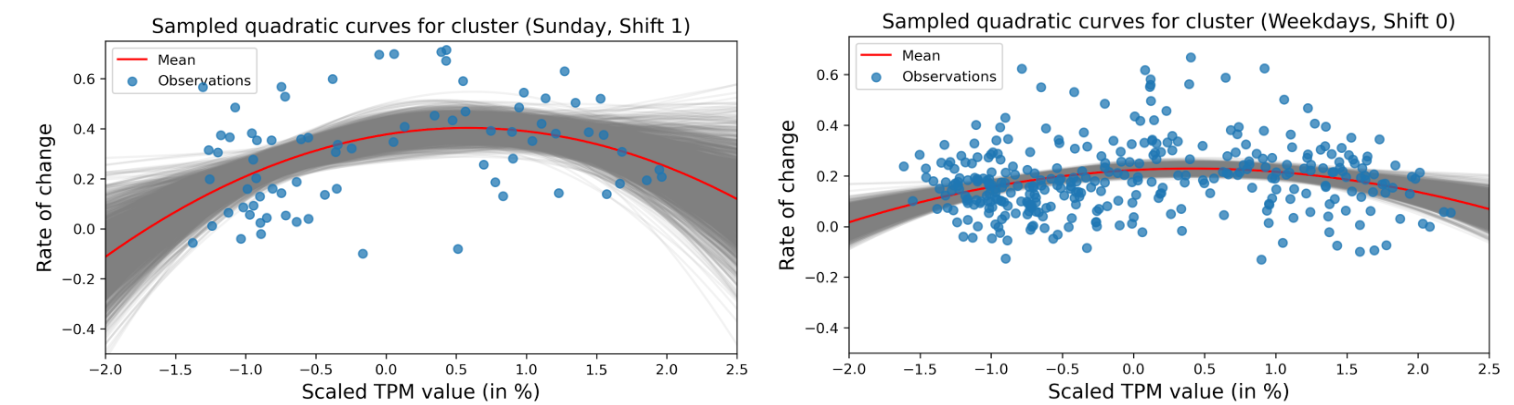
Although BHM is generally quite expensive numerically, this did not play a role in our use case due to the small amount of data. Our BHM approach offers several notable advantages. Its hierarchical structure allows us to include information from other groups and frying pans in the training process, which becomes particularly valuable when dealing with a new frying pan with limited or no available measurements. Moreover, the model provides a direct way for incorporating uncertainty estimation into the model-building and prediction process. It is able to directly compute the probability of a threshold violation in the upcoming hours.
Model Results
Several time series data from different frying pans are arbitrarily chosen to train and evaluate the models on their respective training and test sets using the ROU evaluation method, as the differences to the computationally more demanding ROR method were neglectable For shorter time series with only a few measurements, ROR would be more suitable as a methodology since it expands the training set over time. Our results were summarized in a CM to compute accuracy, prediction, and recall. The table below shows how these metrics for the statistical models differ from those of the ODE baseline model in percentage points (pp).
| Accuracy | Precision | Recall | |
|---|---|---|---|
| SLM | +5 pp | +30 pp | +24 pp |
| BHM | +5 pp | +27 pp | +30 pp |
Among all three metrics, the SLM and BHM have higher values compared to the ODE approach. The accuracy of the BHM is equal to the accuracy of the SLM. While the BHM outperforms the SLM regarding the recall, it exhibits a lower precision than the SLM. Therefore, the BHM detects more of the threshold violations but also predicts more false positives compared to the SLM.
The following figures depict two exemplary episodes, including the forecasts from all three model approaches, to show which scenarios are more challenging to forecast. The episode on the left illustrates a relatively regular curve, whereas the one on the right displays an irregular pattern with intermittent drops in TPM values. This indicates cases where employees are likely to have topped up or partially replaced the frying oil, leading to unexpected fluctuations in the TPM value. In such scenarios, predicting the subsequent TPM value becomes much more difficult due to the lack of information about the employee’s behavior.

Conclusion
Reflecting on our project, we have demonstrated how mathematical modeling can significantly impact operational efficiency, cost management, and food safety in the restaurant industry. We showed the importance of selecting the right models and metrics for our specific use case, modeling the frying oil degradation, and forecasting violations of the TPM limit. In particular, we have emphasized the importance of quantifying uncertainties directly at the modeling stage, as we want to be able to directly control the probability of exceeding the TPM limit.
For our specific use case, the BHM model is the most attractive, as it also allows more accurate predictions in the case of new frying pans with little or no prior data compared to SLM. Furthermore, the quantification of uncertainty is at the heart of Bayesian modeling. We look forward to extending this model in the future to provide even greater benefits for the food safety sector.