Grafana Annotations with Prometheus (a Deep Dive)

Grafana is often used in conjunction with Prometheus to visualize time series and compose dashboards for monitoring purposes. A variety of data fits really well into time series and can be visualized as graphs – such as request count, request duration or response size. Other data is more event-driven and does not quite fit in a graph – for example process restarts, config reloads or the deployment of a new release. The latter tend to happen less frequently and most of the time you would be looking at a flat line if you dedicate a graph for them. However, the events are still interesting to monitor and to correlate with the graphs. For example, a config reload of a malfunctioned config could explain a drop in requests. A nice way to do that in Grafana is to use annotations.

In this blog article, I will dive deep into the specifics of annotations and how to use them with Prometheus as a data source.

What are annotations?

Annotations are descriptions of points in time which can be added to dashboards. They show as vertical lines in the panels and, when hovering over them, reveal a descriptive text and optionally a set of tags. Annotations can be technical or non-technical. For example, an annotation can be created for the start of a new marketing campaign in order to monitor its effectiveness by looking at the incoming requests. Annotations can be created manually, either directly in a panel or using the API. They are stored in Grafana’s database and are associated with the dashboard in which they were created. By default, annotations are only shown in the dashboard in which they were created. However, annotations can also be queried and displayed using a tag selector. Annotations are shown on all graphs of a dashboard. Support for annotations on a single graph are discussed here.

Grafana also has support for region annotations. They have a start and end time (which is different from the former) and the region in between is shown in a slightly different color on the panels. They can, for example, be used to denote an outage or the lifetime of a job.

Manual annotations work well for non-technical events or to enrich graphs after a debugging session. However, it would be cumbersome for automated events. To that end, Grafana allows to query annotations from external data sources. Multiple data sources and queries can be defined per dashboard. They are visualized in different colors and can be individually hidden by a toggle switch at the top of the dashboard. We will have a closer look at querying Prometheus for annotations.

Annotations from Prometheus

Data returned by Prometheus can be used to show annotations. As a prerequisite, Prometheus has to be configured as a data source in Grafana. To show time series in Grafana you have to specify a PromQL query. Annotations use that same query language. But how does Grafana transform the time series into annotations? Prometheus has no concept of annotations. Unfortunately, this feature is not well documented. I had a browse through the code and share my findings here. If you are not interested in the technical details, skip to the next section to find some examples for inspiration.

To get started, go into the dashboard settings of your dashboard and choose “Annotations“ in the menu. It will show you all existing configurations, however, we want to create a new one by clicking “New“. The settings “Enabled“, “Hidden“ and “Color“ give us some options to manage a multitude of annotations more easily. We leave those settings as they are in this example. When Prometheus is properly configured, we can choose it as a data source here. Afterwards, we can specify a search expression, i.e. a PromQL query. Grafana performs a range query for annotations. That is, our PromQL query returns a vector of time series where each element covers the time range of the dashboard. Of the response, each time series is processed independently. Grafana considers all non-zero and non-null values for annotations. The remaining data points are gaps. Every non-zero and non-null data point which follows a gap denotes the beginning of a new annotation. All subsequent data points belong to the same annotation (which would make it a region annotation), until the next gap is reached.

Let us consider an example. Suppose we want to monitor Prometheus alerts. Fig. 3 shows the required configuration. Fig. 2 shows a sample annotation.

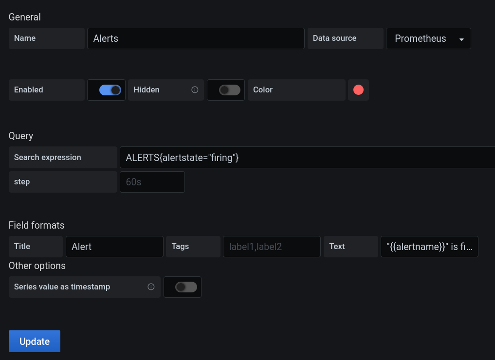
The “step“ option can be used to change the resolution of the query (it is passed to Prometheus’ range query API). The default is 60s. The setting is independent of the selected time range of the dashboard, with one exception. If the range query reaches Prometheus’ maximum allowed data points of 11000 per time series, then the resolution is reduced to stay in bound of this limit. The static step size is different from panels, which adapt their resolution to avoid unnecessary expensive queries against Prometheus.

The appropriate setting for steps depends on the type of event you are trying to obtain from the time series. It is a tradeoff between performance and integrity. If the resolution is too low an event might occur between two data points or two independent events might be merged because the gap between them is not sampled.

Another aspect to consider when choosing the right value for the “step“ option is the visualization. With too many annotations in a small window, all the horizontal lines take away the focus of the underlying graph. Grafana only shows one annotation per step. That is, the lower the step size, the fewer annotations can potentially clutter the panels. The annotation configurations can be reordered to give priority to certain annotations.

To keep the number of annotations manageable but still avoid missing an annotation you can make use of Prometheus’ range vectors (not to be confused with range queries) in conjunction with a high step size. Range vectors must be aggregated over time before querying. A common use case is to calculate the rate of some counter. If that rate is mostly zero, it might be well suited for an annotation. A good example is the restart of a process.

If you choose a step size and range of 30 minutes, there will be at most one of those annotations in an half hour interval. On the downside, the time of the annotation may be off by 30 minutes and you don’t know how many restarts occurred.

Each annotation has a title, a text and a set of tags (see Fig. 1). The title and text are templated strings. They can include labels from the time series. The tags are sourced from label values, given a list of label keys. As of now, tags of external annotations are only displayed. There is no query or filter ability. Limited string manipulation for all annotation fields can be achieved by levering Prometheus’ label_replace().

By default, the values of the time series are only regarded to distinguish gaps (i.e. zero values) from annotations. Their actual values are of no further interest to Grafana and are not available for templating. However, some components export metrics where the value is a timestamp. To that end, Grafana supports taking the timestamp from the value by ticking the “Series value as timestamp“ option.

Let’s look at an example. The kube-state-metrics exporter exposes the creation time of a pod as a metric. We can use that to visualize the creation of pods as annotations.

There are a few things to consider here.

• Grafana expects the values in milliseconds. By convention, Prometheus uses seconds, hence, we multiply by a thousand.
• The time series kube_pod_created only exists for the lifetime of the pod. That means, to appear as an annotation the time series must be returned by Prometheus with at least one data point (the time series is constant over its lifetime). Even if the timestamp is taken from the value, Grafana still performs a range query. Hence, as long as the lifetime is longer than the configured step size the annotation is sampled.
• If the time series “appears“ when the pod is created, why not just use the timestamp of the time series? This might be sufficient in some cases and, in fact, is a good workaround if no such time series is available. However, it comes with some drawbacks. First, you have to adapt the query to detect the rising edge, otherwise the annotation will become a region annotation. Second, the exported timestamp gives you a much more accurate representation. Third, if the exporter is down, then the metrics will show much later in Prometheus or might contain gaps, which is not a problem if you take the timestamp from the value.
• The example metric we used here has a constant value, the creation date never changes. What about time series that do change, for example a predicted end time? The behavior of this scenario is not documented and a quick look at the code reveals that Grafana does not properly handle this scenario in many cases. Timestamps are processed in the order in which they appear in the time series. This messes up the calculation of region annotations if the timestamps are non-monotonic. Also, there is no way to only take the last value of a time series, because Grafana always performs a range query. TL;DR If you want to stay in safe waters, only use constant timestamp metrics.

A commonly used feature in Grafana are variables. They can be used to abstract particular aspects of dashboards and make them more flexible and versatile. Variables are defined in the dashboard settings and can be referenced in panels to customize their queries. The same works for annotation queries. For example:

Useful annotations

Which annotations you want to show depends on your needs. Here are a few examples to get you started.

Prometheus Alerts

If you manage your alerts in Prometheus, it would be nice to see them in Grafana as well.

The labels from the alerts are available for filtering and templating, for example by component. Alerts will be displayed as region annotations for the period in which they are firing.

Pod restarts

Process restarts might be the cause of a service degradation. If you operate in a Kubernetes environment, restarts metrics are exposed by kube-state-metrics.

We have to detect an increase, therefore we need a range vector. The range should correspond to the configured step size to avoid duplicates or undersampling. Furthermore, each range must contain at least two data points – an increase cannot be calculated from a single data point.

Config reload

A misconfiguration can introduce problems. This query plots an annotation for every change in the configuration of Prometheus.

The range should correspond to the configured step size to avoid duplicates or undersampling.

Creation of a pod

This query shows an annotation for every pod that is created.

Make sure to enable the option “Series value as timestamp“. Grafana requires the timestamp in milliseconds.

Conclusion

Prometheus is not about exact measurements and as such is not primarily built for events. However, the time series database already carries a lot of data, which makes it an interesting source for annotations. Furthermore, no additional infrastructure or scripting is required in a typical Grafana + Prometheus setup in order to get started with annotations.

PromQL is purposely designed to be lean and built for time series in mind. It hands a lot of responsibility to Grafana. Grafana has put a lot of flexibility in panels (check out transformations introduced in Grafana 7.0) but those are not available for annotation queries. As a result, querying annotations using PromQL is a bit hacky.

There are a few interesting feature requests regarding annotations, for example better support to deal with many annotations. You can find all the discussions around annotations on GitHub. Grafana is developed in the open. Feel free to join the discussion and contribute.