From Exploration to Production — Bridging the Deployment Gap for Deep Learning

This is the first part of a series of two blogposts on deep learning model exploration, translation, and deployment. Both involve many technologies like PyTorch, TensorFlow, TensorFlow Serving, Docker, ONNX, NNEF, GraphPipe, and Flask. We will orchestrate these technologies to solve the task of image classification using the more challenging and less popular EMNIST dataset. The first part introduces EMNIST, we develop and train models with PyTorch, translate them with the Open Neural Network eXchange format ONNX and serve them through GraphPipe. Part two will cover TensorFlow Serving and Docker as well as a rather hobbyist approach in which we build a simple web application that serves our model. You can find all the related source code on GitHub.

Bridge the Gap to Move towards an AI-powered Society

Andrew Ng is an artificial intelligence rockstar. Being professor at Stanford, co-founder of Coursera and deeplearning.ai he tremendously pushes AI education and application. He can be assumed to be the teacher with the most students in this field which earns him great authority. With this he coined the term of AI as the new electricity that lights a new industrial revolution. But, in contrast to the ease of this claim it took massive efforts to take electricity from labs to millions of households and factories. It took manpower, heavy investments and practical solutions to take it from theory into practice and make it a matter of course for the masses. And Andrew Ng also knows about this.

With AI — going back to his analogy — the case is similar. There is a myriad of research in AI and there is also growing practical application, in healthcare, transportation, or commerce — just to name a few. However, most people are still far from actively perceiving AI as an integral part of their daily life. There may be political, societal or cultural factors slowing adaption. To be fair, we also need to be more precise about what we mean when talking about Artificial Intelligence. This distinction between narrow and general AI illustrates that we haven’t passed the point of what many people mean when they actually talk about AI.

Either way, to solve lacking mass engagement and understanding, we need to make AI more accessible. In his speech at the AI Frontiers Conference in 2017 Andrew Ng shared his vision of an AI-powered society and the need to give people all the tools to make that vision becoming reality. In my view, this goes hand in hand with better bridging the gap between exploration and production. With this I mean the steps to take a machine learning model from its concept and development stage to deployment. Model deployment brings models to life, makes them accessible for the masses and allows us to see their realistic performance. Staying with Andrew Ng’s analogy we can compare exploration-translation-deployment of AI with generation-transportation-consumption of electricity. To empower people to do this and bridge the gap, I decided to write a blogpost that incorporates different technologies along the way from exploring to deploying neural network models.

EMNIST Image Classification Models with PyTorch, Translation with ONNX, Deployment with GraphPipe

For this exploration-to-production tutorial, we will solve a supervised learning task with neural networks and serve predictions through a web service. We split this into the following 4 steps:

• Data Exploration
• Model Development
• Model Translation
• Model Deployment

Starting with the exploration phase, I will first introduce the EMNIST dataset and outline its characteristics. Secondly, we continue with building and exploring neural networks to learn a proper mapping between input and output by assigning correct digits and character labels to images. A few iterations will quickly provide us with a satisfactory accuracy level. Just notice: I will not cover data science topics in detail here as this is not the focus of this blogpost, so data and model exploration will be rather superficial and further model tweaking is left for you. Third, it becomes time to leave the lab and roll up the sleeves: therefore, we translate the model into a framework-independent representation. In the final part, we import this representation and turn it into a deployable model and configure the inference interfaces to make it available for users.

Data Exploration: the EMNIST Dataset

The MNIST dataset of handwritten digits is the de facto Hello World for data science (among Iris flower data and Boston pricing). EMNIST is offered by the US National Institute of Standards and Technology (NIST). It extends the digits by images of handwritten characters — uppercase and lowercase. With 28×28 pixels and a single color channel (greyscale) the images have the same format as in MNIST. The whole dataset contains 814,255 images from 62 classes (10 digits, 26 lowercase and 26 uppercase characters). For those of you that are interested in more details, have a look at the corresponding paper from 2017. MNIST has become really widespread for all kinds of deep learning tutorials due to its easy accessibility, limited size and easy to grasp structure. However, it has also become overused in my view. Therefore, I decided to take a step further for the practical part of this blogpost that is not too far from existing content, but far enough to add some diversity.

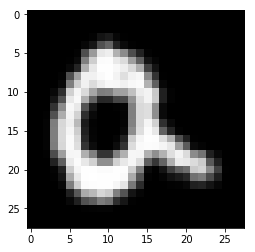
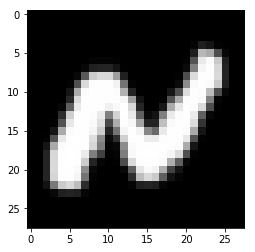
NIST offers the EMNIST dataset in two different formats: binary and Matlab. I decided to stick with the Matlab format and if you like to take the same road, you are welcome to use the proper loaders. Reading the images and labels provides us with 697´932 training and 116´323 test examples which is almost a 6:1 train-test split that we keep here. Below, you can see some examples from the dataset:

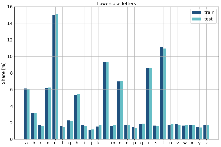
A problem that comes with EMNIST is the highly unbalanced class distribution. Not only between digits and letters, but also within letters. Thus, the 10 digits constitute about half of the instances in both, training and test datasets. Within letters there is also a large disbalance in two ways. First, across upper- and lowercase letters. This particularly applies to some of the most frequently used letters in English language like e, s, t or o. Secondly, within upper- or lowercase letters there is a large disbalance reflecting this differing usage frequency in language. Nevertheless, there is a good aspect left. The letter shares stay approximately constant when we compare train with test data distributions.

This unbalanced data can impede classification models from correctly learning the right pattern-to-label matching. There are plenty of methods with their pros and cons to anticipate this. We can downsample classes to achieve a uniform distribution. We can upsample data by duplicating underrepresented class instances or creating synthetic samples. But, we can also adjust our later training loss calculation in a way such that underrepresented classes receive higher weights such that classification errors equally affect the loss regardless of their underlying frequency. But, staying with my remark, this should be none of our concerns here.

Model Exploration: Develop Neural Network Models with PyTorch

Following our first impression of the data we can start exploring useful models. This is generally an iterative process that involves building a model, training it and assessing its performance on our test data to estimate its generalization capacity. Afterwards, we select the best one(s) and bring them into production.

A short Excursus on how we can fail in Data Science

This process also involves a lot of failing which is absolutely fine if you fail fast and learn quickly. Therefore, I generally distinguish between three kinds of failing:

• technical
• mathematical
• performance-wise

Technical failing is due to incorrect usage of an API leading to uncompilable models or runtime errors. For example, implementing a fully-connected layer in a neural network, we have to define the number of units the layer’s weight matrix expects and the number of output units. If we now stack this layer on top of an input layer that does not meet the defined dimensions the model definition process or instantiation will lead to an error. This kind of problem category is normally straightforward and more or less easy to detect and correct. It concentrates on the implementation of an existing concept for a model that we have in mind.

Mathematical failing can become more complicated to identify and fix. Models that show mediocre prediction quality due to high bias and / or high variance mostly fall into this category. This means that a model is correctly defined and successfully runs on training data — from a technical point of view — but leads to illogical or totally poor results which makes us believe that the model is learning no proper mapping from input to output data. We may attribute these problems to adverse hyperparameters or inadequate model architectures. For example, we can choose a learning rate that is too high and see our loss functions heavily oscillating instead of converging. These kinds of problems generally involve more intense cause analysis and sometimes a lot trial-and-error. Their solutions also benefits a lot from experience, domain knowledge and solid understanding of theoretical foundations.

Performance-wise failing characterizes the models that fall short of our expectations. These expectations can be quality- or efficiency-oriented and relate to classification accuracies, the tolerable amount of false positives, but also training duration, model complexity or inference times with respect to later scalability. In this highest stage of failing, we see models that are technically correct and that successfully learn from our data. But we are still unsatisfied with what or how they learn. For example, we may train a shallow neural network on images to classify them correctly and our model converges at 60% classification accuracy. Thus, we are probably unsatisfied with its results and may increase the model complexity to improve on the accuracy.

Selecting the right Deep Learning Framework

As we can see, a model needs to pass different quality gates. Generally, it takes many iterations to drive our approach to pass through them. Especially for beginners, I would therefore recommend using frameworks that support fast failing and learning as well as supports our understanding of why we fail. When I started building my first neural networks TensorFlow was at version 1.0. Now we are approaching version 2.0. It is the most widely adopted deep learning framework with a strong community and supported by Google. I got used to the sometimes rather un-pythonic way of solving problems with it. As opposed to it, PyTorch has become a strong competitor with also large support from the community and backed up by Facebook. Where TensorFlow stands as the mature framework with useful features like TensorBoard for visualization and TensorFlow Serving for model deployment and production, it also suffers a little from its static graph paradigm which can slow down failing and learning. Here, PyTorch better integrates with the Python data science ecosystem and uses a dynamic graph paradigm that lets you easily and quickly explore variables and respond to failures. Nevertheless, it’s missing some functionality and maturity and one also has to mention that TensorFlow is anticipating the dynamic graph with its eager execution mode that is announced to become “a central feature of 2.0“. I took this blogpost as a chance to become more acquainted with PyTorch and in particular to explore how we can get the most out of different worlds. Doing so, I will focus on TensorFlow and PyTorch as the two most significant frameworks and refrain from comparing other frameworks like CNTK or Caffee.

Modeling Neural Networks in PyTorch

Back to EMNIST and our problem of digit and letter classification:

In this section, we build two different models and train them on the EMNIST training dataset. First, a simple linear model that fully connects input to output units and applies a softmax function to the output units to predict the class that relates to the highest output value. Secondly, we increase the depth of this shallow neural network by adding two hidden layers which are also fully connected to each other. As loss function, we use the mean cross-entropy. To back-propagate the loss and perform the gradient updates, we use the Adam-Optimizer which uses an adaptive momentum for the gradually diminishing learning rate within stochastic gradient descent. Furthermore, we use mini batches with 128 images each and train for five epochs. After seeing my Jupyter notebook kernel die having almost 100 GB compressed memory, I decided NOT to use all testing instances for evaluation, and rather sampled a random subset of 5% to use for each evaluation step. Nevertheless, we should use the whole test dataset and evaluate batch-wise to get a more reliable perception on the generalization capacity of both models after we trained them. Refer to this notebook for the code and to try it yourself.

Linear Model

First, we load our EMNIST dataset and set some informative variables for our latter training procedure:

Next, we easily create PyTorch tensors as basic data building blocks from our NumPy Arrays. This also shows the nice integration of PyTorch. In addition, we normalize the pixel values of our grayscale images to the unit interval and flatten them. In PyTorch, we don’t have to one-hot encode our labels for classification tasks. This is internally handled by PyTorch. The only thing we have to take care of here is to provide them in integer format:

Now, we define the linear model as a new class that inherits from torch.nn.Module. We usually define the model in the constructor and override the forward method. During training we pass it input data, it performs the forward propagation and returns the results of the output layer. This is a minimal configuration for a model in PyTorch with easy extendability as we will see in the second model:

After we set up our model, we create a model instance and define the loss function (the criterion to minimize). Furthermore, we set up the Adam optimizer by passing the model parameters and a proper learning rate for the optimization process:

To control the length of our training, we define the number of epochs, i.e. full passes through the training data, along with a proper batch size which is the number of training instances that are used for a single iteration. In order to track and visualize the model performance throughout training, we also provide some lists that keep losses and accuracies for both, training and test dataset. Finally, we also define the frequency of evaluations:

Finally, we set up our training routine that runs through the epochs and batches respectively. Every iteration, we draw a batch from the training data, reset the gradients accumulated before, perform a forwards pass to obtain predictions and compute the loss resulting from the deviation between predictions and true values. We backpropagate this loss by calling the backward() function on it and perform a parameter update that adjusts the network’s parameters accordingly. Optionally, we take the current model and apply it to the test data to track its progress and estimate the generalization performance. Now we are all set to start the training procedure.

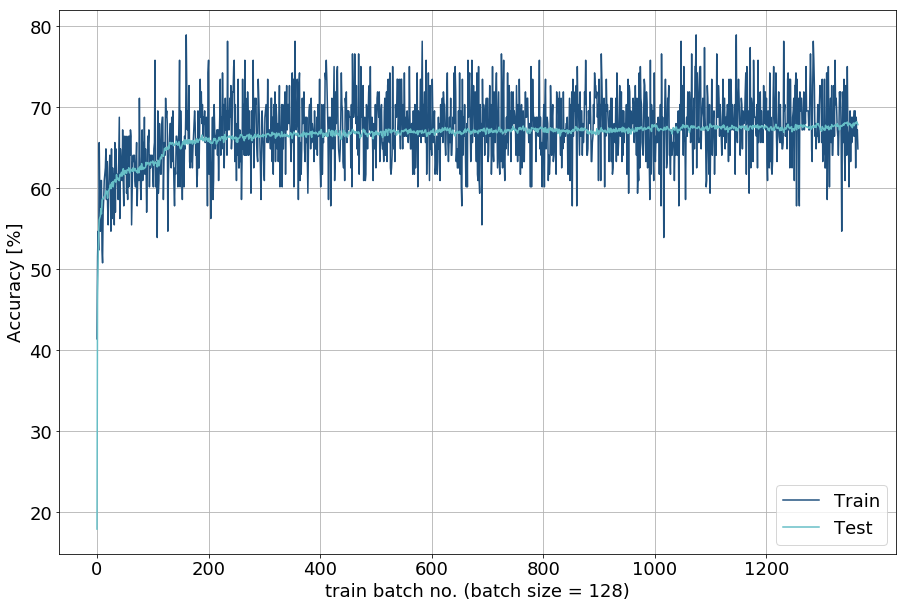
Here is what we get from it: the test accuracy converges to about 68%. Normally, we would now step into some deeper error analysis, for example by identifying for which classes the model was particularly wrong consulting the confusion matrix or by adjusting our loss function weighting underrepresented classes according to their inverse frequency.

In order to illustrate how easy it can be to extend from existing model definitions in PyTorch, I will rather extend the existing architecture to a deep neural network by adding two hidden layers. Without a respectable discussion on what constitutes DNNs to be actually deep, let’s go for it and simply adjust our network a little. However, if you like to be prepared, consult Goodfellow, Bengio and Courville here.

Deep Neural Network

Once we set up the surrounding parameters and tracking capacities, exchanging or adjusting models is pretty easy. We may define further classes based on existing or define totally new models following the structure that was already shown above. Thus, we similarly define a DNN by just extending the number of layers as well as defining the operations that connect those layers with each other. Here, we apply the exponential linear unit function to activate the logits of the hidden layers.

Finally, we observe the DNN to achieve more accurate classification results as the linear model. Thus, we stick to the more accurate model as it performs significantly better on the test dataset with an approximate accuracy of 78%. his performance serves as proxy for generalization capacity and we want to use models that we expect to generalize well on new data.

Of course, these results are far from being really satisfying and rigorous, instead they serve illustrative purposes. We could extend our approach with hierarchical model structures that first distinguish digits from upper- from lowercase letters and do the recognition secondly. We could also shift to using convolutional neural networks. However, the focus here is not model tweaking and exploration, the focus is to better connect exploration with production. Thus, we finish model development at this point and proceed with the model translation.

Model Translation: Using ONNX — the Open Neural Network eXchange Format

After model exploration and selection, we have to consider how to put the model into production. Deploying framework-dependent models can be challenging. In general, there are two paradigms to approach this on a higher level: on the one hand, one can stay with the framework that was used for modelling and training, for example by implementing a web service that embeds a forward propagation. On the other hand, one can cross framework-boundaries and mix technologies. I personally prefer to use the best of different worlds and hope to convince you to do the same — with ease and some guidance. With that said, let’s cross the gap and move beyond boundaries.

First, we elaborate on some criteria for machine learning model deployment in production:

• High-performance and Scalability
• Flexibility
• Interoperability
• Maturity

The solution needs to deal with concurrency and frequency of requests and serve them at high speed regarding transmission, preprocessing, forward propagation and post-processing. If resources deplete, further need to quickly scale to the incoming demand, especially with respect to fault tolerance (reliability). Flexibility refers to language support, configuration and model handling. Interoperability relates to supporting multiple frameworks and formats with the least effort. Finally, maturity can pay off from the very beginning if some criteria are not fulfilled. Maturity fosters adoption which promotes discussion, problem solving as well as the diversity and quantity of ideas. This make it easier to start with something new. Nevertheless, its not crucial if the solution is already very good at some points which may compensate sufficiently in the beginning when there is few adoption.

Open Neural Network eXchange format (ONNX)

ONNX stands for Open Neural Network eXchange format and claims to be the “new open ecosystems for interchangeable AI models“. It provides a standard format to represent deep learning models and allows interoperability by easily sharing models between frameworks. It is supported by Amazon, Facebook and Microsoft and exists since 2017. The ONNX format defines a computational graph model. There are many tutorials referenced on their GitHub page for exporting and importing from and to different frameworks. Caffee2, Microsoft Cognitive Toolkit, MXNet and PyTorch natively support ONNX. There are also connectors for TensorFlow and CoreML. And with the TensorFlow 2.0 announcement pointing out the “standardization on exchange formats“ we may also hope for TensorFlow natively supporting ONNX soon. However, we can see some rather hesitant reactions from officials in this ongoing discussion on GitHub. In general, ONNX can be seen as a modern, accessible and deep learning focused successor of PMML, the Predictive Model Markup Language (PMML), which is used to represent predictive models along with data transformations in a framework-unspecific way.

Fortunately, PyTorch has already integrated ONNX and thus provides functionality to export models into ONNX protobuf format. Therefore, we export our model with torch.onnx.export and pass it the model, a path where to save it and an example input. Since the model export itself works via tracing we need to provide this example input. This means that invoking the export triggers the model to perform a forward pass using this input and records a trace of operators that were involved in computing the output. Thus, the example can also be random data, but needs to match the shape we specified for model input. Finally, we may also specify names for model parameters. Now, we can apply it to the trained deep neural network dnn_model to obtain the export file:

Model Deployment: GraphPipe and Docker for Efficient Model Server Implementations

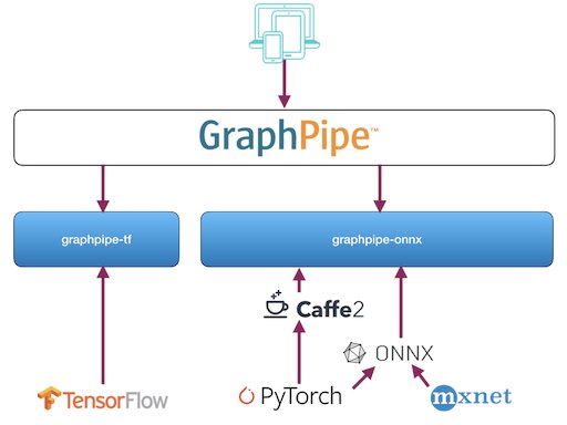
Oracle recently published GraphPipe to “simplify machine learning model deployment and decouple it from framework-specific model implementations.“ GraphPipe’s machine learning transport specification uses Google’s flatbuffers. It provides reference model servers for TensorFlow, caffee2 and ONNX as well as client implementations for Go, Java and Python. Integrating ONNX support broadens its support for even more deep learning frameworks. Although it accepts ONNX as a framework-independent model format, GraphPipe uses framework-specific model servers. Tweaking the model server configurations and standardizing client-server communication, GraphPipe excels in server efficiency and performance. Respective model servers come embedded into Docker containers offered on their website. The ONNX model server accepts ONNX models as well as models in caffee2 NetDef format. The TensorFlow model server handles both TensorFlow models, the SavedModel and the GraphDef format. Here is a summary of how a GraphPipe handles a request:

In essence, a GraphPipe request behaves like a TensorFlow-serving predict request, but using flatbuffers as the message format. Flatbuffers are similar to google protocol buffers, with the added benefit of avoiding a memory copy during the deserialization step. The flatbuffer definitions provide a request message that includes input tensors, input names and output names. A GraphPipe remote model accepts the request message and returns one tensor per requested output name. The remote model also must provide metadata about the types and shapes of the inputs and outputs that it supports.

ONNX and GraphPipe are not the only technologies that promote interoperability and deployment ease. Almost at the same time as GraphPipe was released, the Khronos Group published its Neural Network Exchange Format (NNEF) as a new standard to support interoperability. In addition, with Glow — a Compiler for Neural Network hardware accelerators there is another way of transforming models from different frameworks into a common standard. Feel free to check them and don’t forget to share your experiences. For this blogpost, we will concentrate on ONNX and GraphPipe for now on and heading back to the practical part. With this said, let’s get back to our EMNIST image classification model and serve it through GraphPipe. You can refer to this Jupyter notebook for the code.

First, make sure you have Docker installed on your machine. Secondly, pull the graphpipe-tf and graphpipe-onnx container images with docker pull sleepsonthefloor/graphpipe-onnx:cpu and docker pull sleepsonthefloor/graphpipe-tf:cpu . Third, use pip install graphpipe to install the GraphPipe client to test our model subsequently. Consult the user guide for further information. The references are simple to use and let us quickly serve a deep learning model through a running model server. We just go ahead with our ONNX model and start our model server from the root of the repository and using port 9000. In order to do that, we have to create the value-inputs first which are required for serving models with graphpipe-onnx. Unfortunately, the user guide contains very little information on how to set up the value_inputs.json :

However, we can follow the structure for the exemplary Squeezenet input assuming the outer list to describe the batch size per request and the inner list to hold the dimensions of the input:

Now it is time to start the model server with the following command:

Unfortunately, we fail with the following log message (for the complete log, see the notebook):

This seems like some tensor shapes are not set as expected. Nevertheless, without proper knowledge of Caffee2, this can be hard to debug. Therefore, we alternatively try to load both resources (dnn_model_pt.value_inputs.jsonand dnn_model_pt.onnx) directly from GitHub which also fails. Despite the fact that the Squeezenet example worked, trying to replicate this for our own ONNX model is currently a big hassle in GraphPipe. However, with graphpipe-tf as the TensorFlow model server there seems to be a way out. Thanks to ONNX we can easily generate a TensorFlow model export from our ONNX-model and try to serve that one through GraphPipe. Therefore, we only have to install the ONNX TensorFlow connector. Hence, let’s give it another try:

After translating our ONNX model into a TensorFlow protobuf, we start the Docker container with:

Brings the following to our terminal:

This looks much better now. Despite some initial difficulties, we deployed our model quickly in just a few lines of code. That is why we know want to know whether what we deployed behaves similar to what we trained.

Therefore, we finally validate the deployment using some test data queries against the REST interface of our containerized model server. To do this, we use the GraphPipe client implementation which we have already installed: