If you have recently looked at results from papers about Deep Learning-based 3D reconstruction, novel-view synthesis, and other related tasks in visual computing, you were probably pretty impressed by the level of detail to which the results are rendered. Many of those impressive results are achieved by training so-called neural fields. In this article, I want to shed some light on this concept and show you how you can train such a model in a Google Colaboratory notebook on your own.
Towards this goal, we will look at the foundations of neural fields in visual computing and how they are different from prior representation learning approaches involving neural networks. In a Colab notebook accompanying this article, we will implement simple neural fields for image representation from scratch using PyTorch.
Neural Fields
This section is meant to introduce the basic idea of a neural field. It is mainly based on a recently published review paper [Xie et al., 2021], which I highly recommend reading if this blog article gets you excited about this type of network.
Let’s start with two definitions from the review paper about neural fields. The term field is quite overloaded in mathematics and physics. Neural fields are physically inspired, so the definition from physics applies:
A field is a varying physical quantity of spatial and temporal coordinates.
You can think of a field as a function that takes any coordinate in space and time and produces a physical quantity. Depending on the dimension of the field quantity, we speak of scalar fields or vector fields. In a neural field, we use a neural network to parameterize this function. Hence, we feed Spatio-temporal coordinates into our network, which produces the physical quantity for us. In the words of Xie et al.:
A neural field is a field that is parameterized fully or in part by a neural network.
As I am passionate about visual computing, I want to introduce the concept of neural fields by the example of representing images via neural networks. Towards this, let me quickly reflect on representation learning using autoencoders and autodecoders.
Remark: Representation Learning
Typically, representation learning approaches are trained using autoencoder models. The following figure illustrates this concept for the application of reconstructing images of hand-written images from the popular MNIST dataset [LeCun et al., 2010].
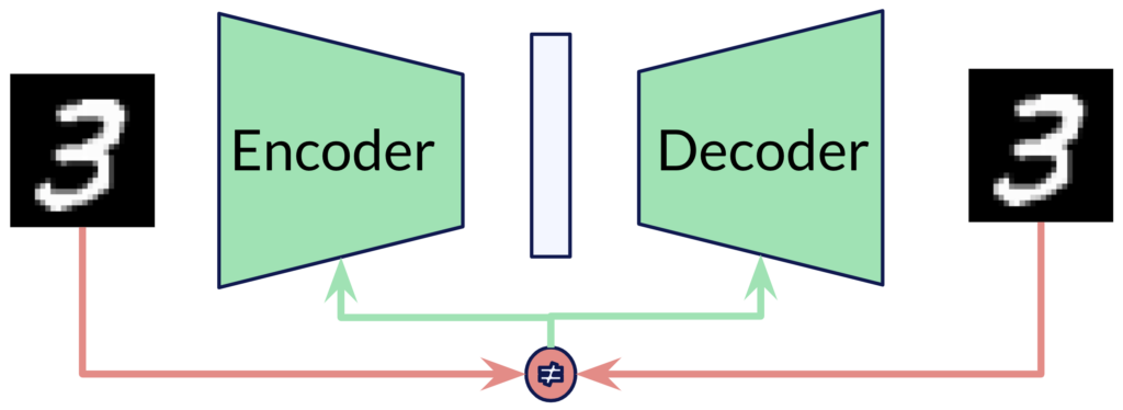
An autoencoder comprises two neural networks. The first network is the encoder, which receives a data sample (here the image of a handwritten digit 3) as input and produces a lower-dimensional encoding of this data sample. The second network tries to invert the process by generating a sensible data sample from the latent code produced by the encoder and is hence called the decoder network. Both networks can be trained jointly by backpropagating the error between the input and generated output. By repeating this process with many data samples, the autoencoder learns to embed the data samples in a lower-dimensional latent space. The goal is to learn a compact representation of the data manifold. An incredible amount of research has been conducted investigating the structure of the latent space learned by such autoencoder networks. It was also discovered that one does not need the encoder network to train the decoder as a generative model. With Generative Latent Optimization (GLO) [Bojanowski et al., 2018] for images and DeepSDF [Park et al., 2019] for 3D shape, two so-called autodecoder networks were introduced that are capable of organizing the latent space without the encoder. The key idea behind autodecoders is depicted in the following figure.
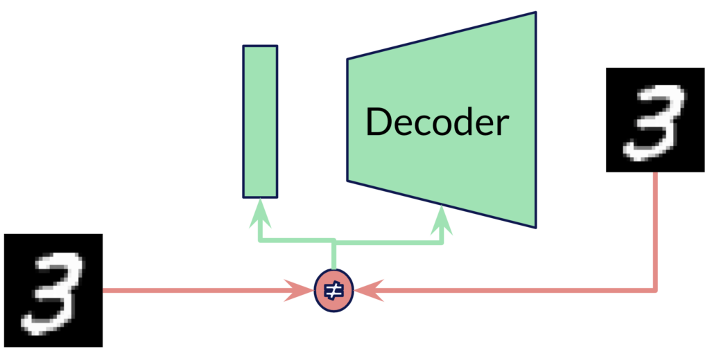
Instead of computing the low-dimensional latent vector for a training sample through the encoder, a learnable vector per training sample is used as the input to the decoder. The values of the vector are updated jointly with the decoder weights during training. At inference time, however, we need another optimization loop in order to find the latent vector for a given sample. A nice side-effect of this is that we can formulate the inference-time optimization over partial observations, hence deploying our trained autodecoder to tasks like image inpainting, or 3D surface completion. But more on that later. First, I would like to draw a connection between autodecoders and neural fields.
Rethinking Data
Let us step back for a moment and think about the autoencoder and autodecoder formulations introduced above. In both cases, the dimensionality and resolution of the input and output are usually defined and fixed at modeling time. Hence, if I train a model to encode RGB images of resolution \(640 \times 480\), the output of my model will always be of that resolution. For larger resolution, I have to adjust the model architecture and hence, the number of parameters of my model grows with the resolution of the images I want to generate. Neural fields are formulated to be invariant to the resolution of their output. Let me show you how this is achieved.
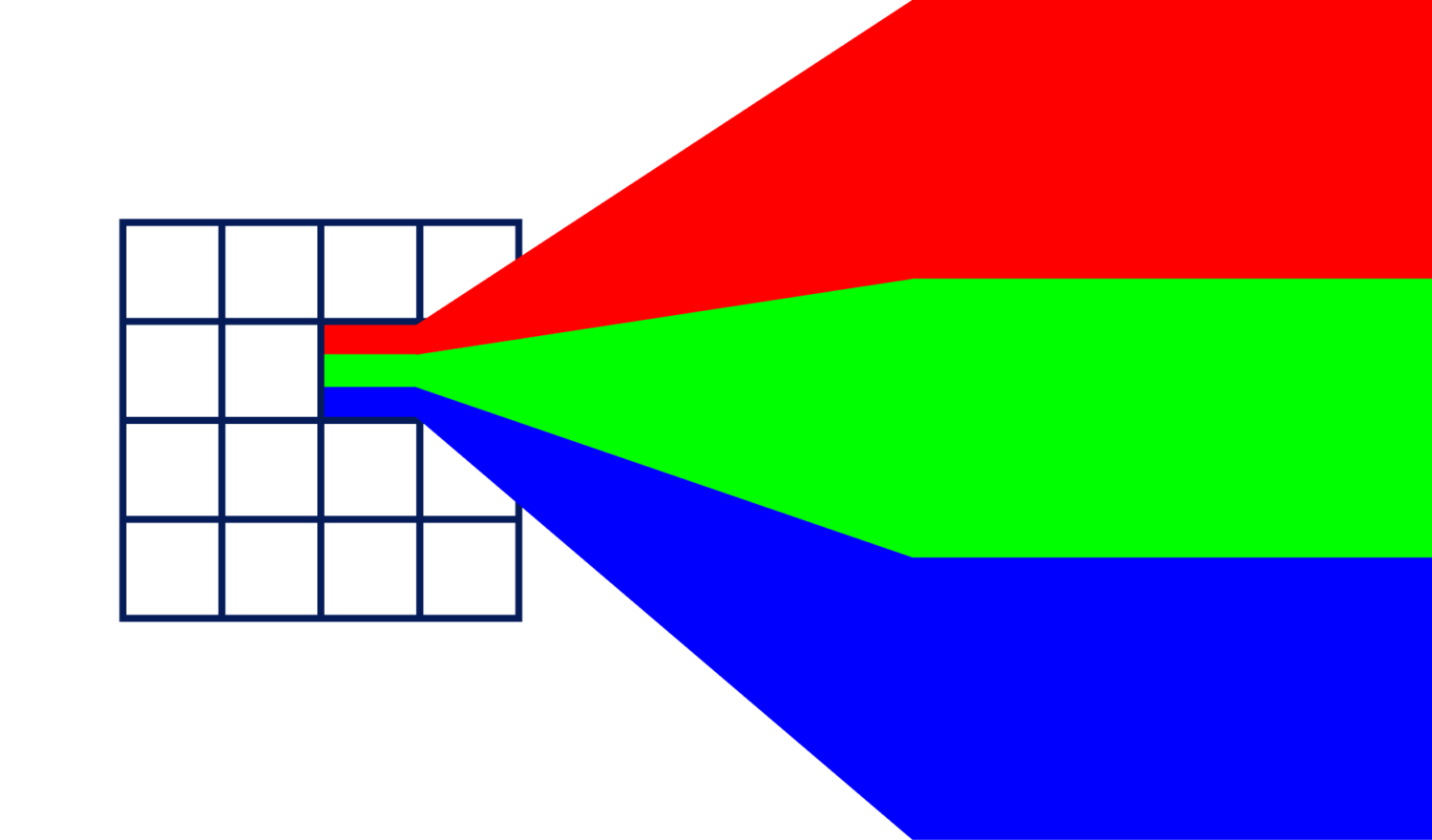
The key here is to think about the data that we consume with our model, which is images in this case, geometrically. Towards this, I will borrow some ideas from the Geometric Deep Learning blueprint by [Bronstein et al., 2021]. Frankly, it goes like this: Images are built out of pixels, which are organized on a euclidean grid. At each location in this grid, we have three numbers encoding the intensity of the red, green, and blue base colors, that are mixed together and compose the color of that pixel that you and I can perceive. For the following discussion, we consider the raw pixel grid as the (geometric) domain \(\Omega \) and the pixel values as a signal (or function) \(x: \Omega \mapsto \mathcal{X} \) that is defined on that domain. In representation learning techniques, we typically fix the domain and learn a function that maps to specific \(x \in \mathcal{X} \) representing concrete images from the training set. Hence, our network \(f \) stems from a hypothesis class \(\mathcal{F}(\mathcal{X}, \Omega) \) defined over the signals and domains and we learn a mapping \(f: (\mathcal{X}, \Omega) \mapsto \mathcal{X} \). The key difference between this standard approach and a Neural Field is that the latter learns the mapping \(f: \Omega \mapsto \mathcal{X} \) directly. In other words, we train our model to predict RGB values from image coordinates. This is visualized in the following image.
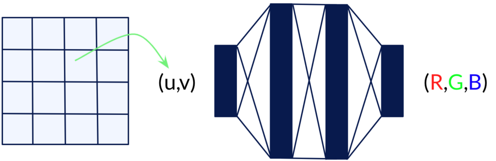
The left-hand side shows the grid, which we will normalize to [0, 1], with continuous values for (u, v). Hence, our network approximates a continuous function, which has several benefits compared to the standard approach to representation learning with autoencoders. First of all, we are no longer limited to a specific resolution, since we can sample the coordinates (u, v) at arbitrary resolution. This also implies that the number of parameters and everything that goes with it (computational complexity, memory footprint, etc.) is independent of the resolution of the images we want to generate. The only limiting factor is the complexity of the signal our network can learn, or in other words, the capacity of our neural network, which we can easily adapt by adding more layers.
Conditional neural fields
The very simple case rendered in the previous section does work well if we only want to overfit a single image. By conditioning the prediction of our Neural Field on additional variables encoding the context, we can use it to represent many images. We can either train our model in an autoencoder manner, or in an autodecoder manner. In both cases, we use the decoder network to represent the Neural Field. Hence, we need to build it in such a way that it accepts two inputs: the coordinates at which we want to evaluate our signal and the latent code that comes either from the encoder or is directly optimized in the autodecoder setting. In the companion Google Colab notebook, we will use the autodecoder formulation. In general, we extend the formulation of our mapping-to-be-learned towards \(f: (\Omega, \mathcal{Z}) \mapsto \mathcal{X} \), where \(\mathcal{Z} \) denotes the latent space from which we sample the conditioning code.
There are also multiple options to implement the conditioning. The straightforward option is to simply concatenate the latent code with the input features and feed the concatenated tensor into the Neural Field decoder. However, using this conditioning technique implies that the network needs to distinguish between input samples based on the input alone. Hence, the first layer is the only one that directly incorporates the condition, while the remaining layers only operate on internal feature representations. There are more sophisticated ideas on how to incorporate the conditioning latent code in a way that each layer (or even each neuron) can make use of the condition. Let me quickly introduce two main concepts which I find very intriguing. The first one is the utilization of a HyperNetwork [Ha et al., 2016], where you take a neural network that predicts the parameters of the Neural Field decoder from the latent code.
Using a HyperNetwork, we actually have a different Neural Field (defined as the decoder network, parameterized by its weights) for each input instance, while in the concatenation-based conditioning, we share the same decoder parameters across all input examples and the distinction between samples must be inferred from the latent conditioning code. Recent basic research in the area of HyperNetworks suggests that the complexity of the primary network (which is the Neural Field decoder in this case) can be much lower, hinting at a more compact representation [Galanti & Wolf, 2020].
A second method is the use of Feature-wise transformations [Dumoulin et al., 2018]. These techniques use small neural networks to predict the layer-wise scale and/or bias vectors that are incorporated in the layer transformation. Two similar concepts are Feature-wise Linear Modulation (FiLM) [Perez et al., 2018] and Conditional Batch Normalization (CBN) [de Vries et al., 2018]. The basic idea is depicted in the image below.
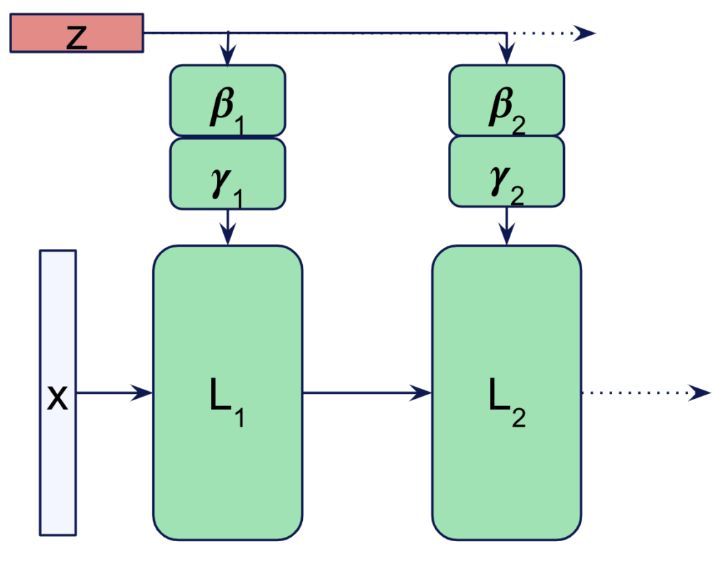
For each layer, we use small neural networks \(\boldsymbol{\beta_i}\) and \(\boldsymbol{\gamma_i}\) to predict scale and bias vectors of the size of the layers output and apply them as: \(\hat{\boldsymbol{x}}_i = L_i(\boldsymbol{x}) \odot \boldsymbol{\gamma_i}(\boldsymbol{z}) + \boldsymbol{\beta_i}(\boldsymbol{z})\).
Global vs Local Conditioning
I mentioned earlier that we provide one latent vector per data sample. This practice is referred to as global conditioning because we encode the whole information about the data sample in one latent code. Likewise, it is possible to spread the information about a data sample over multiple latent codes that are assigned over a subset of the Spatio-temporal coordinates. In this local conditioning, we either assign latent codes for specific spatial regions or time steps. We can also take a hybrid approach, where we use one global code to encode basic information that is shared between instances and several local codes that encode instance-specific details.
Spectral Bias and Fourier Features
This is an excellent time to pause reading this article and jump over to the accompanying Google Colab notebook. Over there, you can go through the code until you have trained the first Neural Field and look at the disappointing results. But hang on! We are about to find out why the results look like they do.
When I execute the first couple of cells and plot the ground truth image next to the network reconstruction, I get something like this:
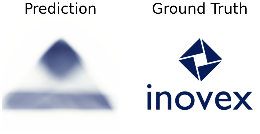
You can try to adjust the number of steps in the training loop and see that you will get the same bad result, even if you let your network learn for many more iterations. There is actually a theoretical explanation for this phenomenon, which is known as the spectral bias of neural networks [Rahaman et al. 2019]. I will not go into too much detail here since the ideas and mathematics involved are very deep and sophisticated. If you are curious, I recommend reading the corresponding papers.
The key takeaway is that neural networks with ReLU activation are biased towards learning low-frequency features first. While Rahaman et al. show this via Fourier Analysis, a different approach to reach a similar conclusion is carried out by [Tancik et al., 2020], who also introduce the Fourier Features as a remedy to this bias.
They use a theoretical tool, called the Neural Tangent Kernel (NTK) [Jacot et al. 2018], which can be used to reason about the trajectory of the neural network parameter updates throughout training. Like many other theoretical foundations of neural networks, the NTK theory considers networks in an infinite width limit. In other words: The NTK theory deals with networks for which the number of neurons in a layer goes to infinity. The reason behind this is that the more neurons we have, the less influence a single neuron’s weight has on the overall network prediction.
If the layer width (and thus the number of neurons) goes to infinity, the individual updates to a single neuron’s weights get infinitesimally small. Consider the network layer function: \(f(\boldsymbol{x}, \boldsymbol{w})\), and the update rule of Gradient Descent for the weight vector \(\boldsymbol{w} \) with learning rate \(\eta \) at time step t:
\begin{equation} \boldsymbol{w}(t + 1) = \boldsymbol{w}(t) – \eta \nabla \mathcal{L}(\boldsymbol{w}(t)) \end{equation}
where \(\mathcal{L} \) is the loss function. If the single update steps are infinitesimally small, we can use the first-order Taylor expansion to approximate the update around the initial weights \(\boldsymbol{w}_0\):
\begin{equation} f(\boldsymbol{x}; \boldsymbol{w}) = f(\boldsymbol{x}; \boldsymbol{w}_0) + \nabla_{\boldsymbol{w}} f(\boldsymbol{x}; \boldsymbol{w}_0)^T(\boldsymbol{w} – \boldsymbol{w}_0) \end{equation}
This approximation is linear in \(\boldsymbol{w} \), but depends on \(\boldsymbol{x} \) in a non-linear way. However, we can use the origin of \(\boldsymbol{x} \) in the approximation above as a kernel function: \(\phi(\boldsymbol{x}) = \nabla_\boldsymbol{w} f(\boldsymbol{x}; \boldsymbol{w}_0) \), which we can use to compute similarities between data samples through the kernel trick:
\begin{equation} k(\boldsymbol{x}, \boldsymbol{x}‘) = \langle \phi(\boldsymbol{x}), \phi(\boldsymbol{x}‘) \rangle \end{equation}
In the infinite width limit, this kernel becomes fixed. But why is this important? Generally, it paves the way to reason about the dynamics of neural networks during training. For example, Tancik et al. show that the eigenvalues of the NTK decrease rapidly for an ordinary MLP with ReLU activations, which means that high-frequency components of the target function (which correspond to the small eigenvalues) are learned very slowly. This explains why we do not see any sharp edges in the reconstructed image of our initial Neural Field! Probably, if you execute the training code on a server and let it run for a few months, you will get nice results, but I guess you do not have the time for that. Besides, there are probably more useful ways to spend your compute resources.
So what is the remedy to this problem? Tancik et al. show that passing the input coordinates through a Fourier feature mapping before passing them into the MLP makes the NTK of the MLP stationary. This is a desirable property for Implicit Neural Representations since the inputs to our MLP are coordinates that are evenly distributed over the domain 𝛺. So let us have a look at the proposed Fourier Feature mapping. The idea is to project the d-dimensional input coordinates \(\boldsymbol{x} \in [0, 1]^d \) to the surface of a hypersphere through a set of sinusoids. In its basic form, the mapping looks like this:
\begin{equation}
\gamma(\boldsymbol{v}) = \begin{bmatrix} a_1 cos(2\pi \boldsymbol{b}_1^T\boldsymbol{v}) \\
a_1 sin(2\pi \boldsymbol{b}_1^T\boldsymbol{v})\\
\vdots \\
a_m cos(2\pi\boldsymbol{b}_m^T\boldsymbol{v})\\
a_m sin(2\pi\boldsymbol{b}_m^T\boldsymbol{v}) \end{bmatrix}
\end{equation}
and induces the following kernel function:
\begin{equation} k_\gamma(\boldsymbol{v}_1, \boldsymbol{v}_2) = \gamma(\boldsymbol{v}_1)^T\gamma(\boldsymbol{v}_2) = \sum_{j=1}^{m} a_j^2 \pi \boldsymbol{b}_j^T (\boldsymbol{v}_1 -\boldsymbol{v}_2) = h_\gamma(\boldsymbol{v}_1 – \boldsymbol{v}_2) \end{equation}
This kernel is stationary (it only depends on the difference between points). Moreover, since we project the points to a hypersphere, we can rewrite the NTK into a dot-product kernel. Tancik et al. show that the frequency decay of the composed kernel \(h_{NTK} \circ h_\gamma \) can be controlled by adjusting the hyperparameters \([ \boldsymbol{b}_1 | \cdots | \boldsymbol{b}_m ] = \boldsymbol{B} \) . By comparing different mappings, they find that the random Fourier feature mapping from [Rahimi & Recht 2007], which samples each entry of \(\boldsymbol{B} \in \mathbb{R}^{m \times d} \) from a Gaussian \(\mathcal{N}(0,\sigma^2) \) and takes the form:
\begin{equation} \gamma(\boldsymbol{v}) = [cos(2\pi\boldsymbol{B}\boldsymbol{v}), cos(2\pi\boldsymbol{B}\boldsymbol{v})]^T \end{equation}
The most important hyperparameter in this mapping is the variance of the Gaussian from which we sample the random matrix \(\boldsymbol{B} \). We will use this mapping in the accompanying notebook. So this is the perfect time to switch back to the notebook and run the training again, but this time with Fourier Features enabled. Look at the following GIF, which shows a snapshot of the image every 25 iterations throughout the training with (right) and without (left) Fourier features applied.
To stress it again: The results above are achieved with the same model architecture. The only difference is the application of the Fourier features, which enable the network to learn high-frequency details early and fast.
Applications of neural fields
So far, we have not really looked into the applications of neural fields. Since we can sample the network at an arbitrary resolution, several image enhancement tasks can be tackled with neural fields. This includes image superresolution, denoising, and inpainting. The underlying domain, which we sample and pass to the network, is shared across all samples our network can represent. The difference between several instances in the dataset is encoded in the conditioning variable \(\boldsymbol{z}\). Using insights from representation learning and generative modeling research, already existing techniques for image generation can be adapted to neural fields and therefore also profit from all the advantages discussed so far. If you think further about generating videos, this means that we can also sample at arbitrarily dense temporal coordinates and hence generate videos with arbitrary spatial resolution and frame rate. Another field that already uses neural fields extensively is computer graphics with 3D content, where you can use the same model, queried at a varying resolution to dynamically adjust the fidelity of the surface details based on available memory, for instance. Also, neural rendering techniques make heavy use of neural fields to render photorealistic images.
Where to go next?
Neural fields are a very active area of research right now, and there is already much more to it than one could cover in a reasonably sized blog article. I nevertheless hope this article serves as a comprehensive introduction. If you want a more complete overview of the topic, I highly recommend working through the very well-written review article from Xie et al. and the accompanying website about “Neural Fields in Visual Computing“. The paper builds a concise mathematical foundation and introduces the terminology that I used in this blog article.
Furthermore, it reviews many more concepts and applications of neural fields. The website provides a collection of recent publications that you can search by keywords, authors, venue, and other criteria. Also, if you have not already looked at it while reading this article, I suggest working through the companion colab notebook to this article, where I provide basic implementations for neural fields in PyTorch.
A comprehensive derivation of Neural Fields in the context of 3D shape reconstruction from partial and noisy 3D observations can be found in the following thesis by the author of this article.