Multimodal Sequential Recommender Systems

Since the invention of the internet, the availability and amount of information has increased steadily. Today we are facing problems of information overload and an overabundance of choices. Recommender systems aim at decreasing the burden of information processing and decision making for end users.

Today’s e-commerce companies rely heavily on recommender systems because they provide significant advantages. Recommender systems help the customer to effectively explore the usually huge product space. Customers need to spend less time until they find what they are looking for. Additionally, the recommender system can suggest new and interesting items to the customer based on the data of other customers. This improves the conversion rate and customer experience. For example, Netflix recently estimated the annual savings through reduced churn caused by their compelling recommender system to be one billion dollars [1] which is about 11.3% of their total revenue in 2016.

Sequential recommender systems are based on sequential user representations \(S^{(u)}_\tau = \{id_1, id_2, …, id_n\}\) for a given user \(u\) and sequence length \(\tau\). Each sequence consists of several items that are represented by their corresponding \(id\) and are given in temporal order. Sequential recommender systems aim at exploiting the temporal information that is hidden in the sequence of item interactions of the given user.

State of the Art Sequential Recommender Systems

In my master’s thesis, I analyzed RNN-based sequential recommender systems. This type of recommender system has two different variants, classification-based models and regression-based models.

One important prerequisite for regression-based models are item embeddings. They transform item IDs into vectors inside a Euclidian vector space. One famous embedding algorithm is Word2Vec, which was invented by Mikolov et al. in 2013 [3]. Its original use case was to transform words into vector representations. The resulting word embeddings are clustered according to their semantic relations. This property of Word2Vec serves as the foundation for the regression-based models. From an abstract viewpoint, a sequence of words is just a sequence of categorical variables. Consequently, this algorithm can also be used for item sequences.

Figure 1 shows the regression-based model of De Boom et al [7]. The user’s item sequence is processed by the sequential part of the recommender system. It consists of an item embedding that transforms item IDs \(id\) into their respective vector representations \(v\). Each item of the sequence is then processed by the Gated Recurrent Unit (GRU) which outputs its hidden state. In this scenario, the hidden state \(h\) corresponds to the user representation vector \(u\), that represents the respective user.

Typically, the goal of a recommender system is to create a recommendation list of length n. Regression-based models consequently select the n items with the highest score.  Here, the score is simply the cosine between the user representation \(u_\tau\) and the target item vector \(v_\text{target}\). The set of all target items usually consists of all items that are in the training set. The process of calculating the score for all target items results in applying a cosine-based kNN which can be seen as an unimodal approach because all items are compared with only one item and the most similar ones are recommended. We can speed up cosine-based kNN by using algorithms for Approximate Nearest Neighbour Search or by filtering the target items by, for example, popularity.

Figure 2 shows the Gru4Rec classification model of Hidasi et al. [4]. It processes the user sequence \(S^{(u)}_\tau \) and directly outputs a discrete probability vector \(p\) whose dimensionality equals the number of items in the training set. In each dimension, the vector \(p\) contains the probability of the respective item to be the next item that the user consumes.

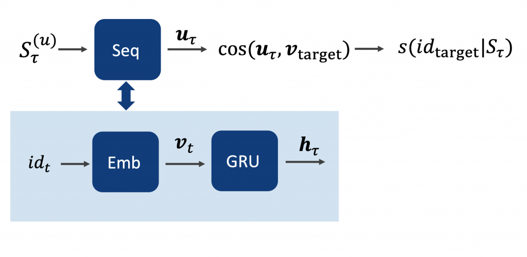
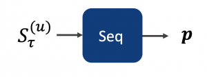
Figure 3 visualizes the unimodal regression-based approach in a 2-dimensional vector space. In this example, the user has already requested two items \(v_1\) and \(v_2\) and is consequently represented by the user representation vector \(u_2\). To create a recommendation list of length 2, the two items with the smallest angle between themselves and the user representation vector are selected.

 

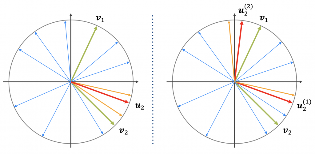
The goal of my master’s thesis was to evaluate, whether a multimodal approach could improve recommendation performance. Therefore, I generalized the unimodal, regression-based model to a model that can represent multiple modalities. Each modality should represent one taste or a combination of tastes of the user. For example, the unimodal model can only represent one user taste  (e.g. Romance films) or a combination of tastes (e.g. Action-Comedy films) that are represented by the location of the user representation vector \(u\) inside the Word2Vec embedding space. It could be beneficial to have a model that can combine different locations in the embedding space and therefore combine multiple user tastes (e.g. Romance and Action-Comedy). Figure 3 shows the idea of such a multimodal approach. The user is now represented by two modalities \(u_2^{(1)}\) and \(u_2^{(2)}\) and their taste should now be more accurately represented.

Methodology

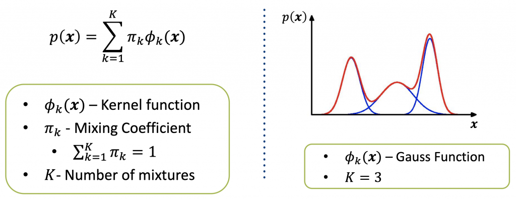
To derive the multimodal model of Figure 3, I took up the idea of mixture models. Figure 4 shows the formula of the general mixture model. The idea behind a mixture model is to model difficult probability distributions as a sum of more understandable distributions. For example, if one chooses the kernel function \(\phi_k\) to be a Gaussian distribution, the resulting mixture model is the famous Gaussian mixture model. Figure 4 shows what a Gaussian distribution with three mixtures could look like. One observes, that it has three peaks and a value \(x\) has an increased probability to be sampled close to the peaks.

It is now well known that there exists a correlation between vector length and word frequency for Word2Vec embeddings [5]. My results and the results of other authors [7] confirm that the cosine-based kNN performs better than Euclidean-distance-based kNN for the unimodal case. Consequently, I decided to derive a novel type of mixture model that is based on cosine.

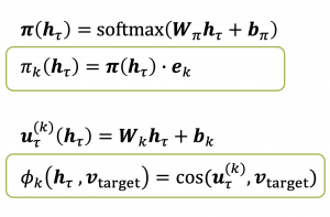
The Mixture of Cosines (MoC) model is inspired by Mixture Density Networks (MDN) [2], which model the means and the covariance matrices of a GMM with multiple-layer Feedforward Neural Networks (FFNNs). The mixing coefficients are modeled by a FFNN with a softmax layer that is trained as a classification network.

The user representation \(u_\tau^{(k)}\) of the MoC model is based on an one-layer FFNN, as shown in Figure 5. The kernel function \(\phi_k\) is then given as the cosine between the user representation and the target item vector. The mixing coefficients are calculated analogously to the traditional MDN.

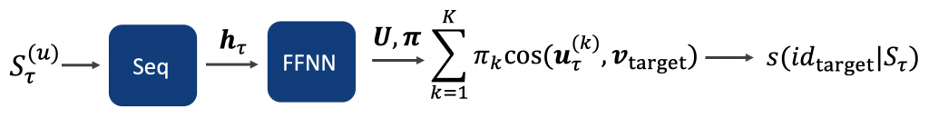
Figure 6 shows a graphical representation of the MoC model. Analogously to the sequential model the user representation \(S_\tau^{(u)}\) is first processed by the sequential part, which consists of an item embedding and a GRU. The final hidden state \(h_\tau\) is then processed by the mixture model part, which is explained in Figure 5. This results in the score for the target item \(id_{target}\).

Results

Evaluation Metrics

To evaluate the MoC model each session of the test set \(S_\text{test}\) is split, so that all items up to the \(\tau -1\)-th item are used to calculate the user representation. Then, a recommendation list of length n is created by selecting the n items with the highest score in descending order.

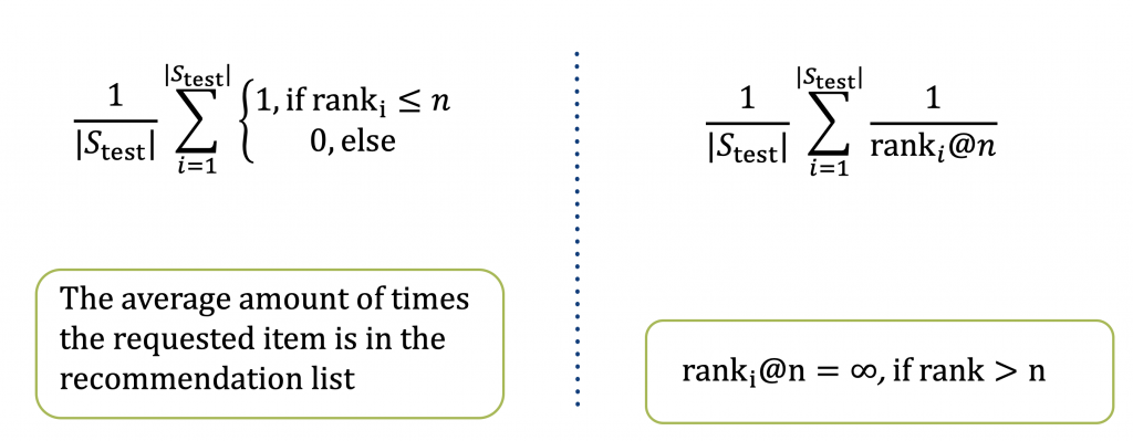
I use two widely used metrics to quantify the recommendation performance: Recall@20 and MRR@20. Both metrics are shown in Figure 6. The rank refers to the position in the recommendation list of the actual item that the user requested. For example, if the item that the user requested is at the third place inside the recommendation list of length 5, then the MRR@5 is \(\frac{1}{3}\) and the Recall@5 is 1. If the rank is 6, then both MRR@5 and Recall@5 are 0 because the rank is greater than the number of items in the recommendation list.

Movielens 20 Million

Table 1 shows the results for the Movielens 20 Million data set [6]. It is provided by GroupLens, a recommender systems research group, and contains 20 Million user-item ratings for 26,744 different movies. The ratings stem from 138,493 different users where on average each user rated 144 and at least 20 movies. Because the type of sequential recommender system that concerns me only considers actions and no ratings, I assume that each rating is an interaction independent of the actual rating. The column G4R refers to the Gru4Rec recommender system [4], a classification based model that represents the state of the art. The other columns refer to the MoC model with the respective amount of mixtures.

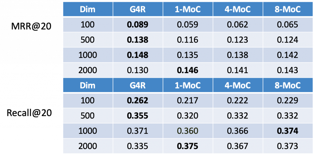
One can see that an increasing number of mixtures increases the performance of the MoC model. However, an increase in the number of dimensions has a stronger positive effect on the recommendation performance. Additionally, the training time with an increasing number of mixtures increases drastically, compared to an increase in the number of dimensions.

Conclusion

I showed that additional mixtures increase the performance of the unimodal model. This increase, however, is rather small compared to an increase in the number of dimensions and the training time increase is huge compared to the gain in performance. Therefore, it is more cost-efficient to increase the number of dimensions of the model than to increase the number of mixtures.

To understand why an increase in the number of dimensions corresponds to an increased modality, one can consider an artificial scenario, where the number of dimensions of the embedding space corresponds to the number of items and each item is represented by the corresponding basis vector \(e_v\). The score of the unimodal model \(s(h_\tau, e_v)\) is given as the cosine, which can be represented as a vector product \(\frac{u \cdot e_v}{|u| |e_v|}\). The vector product can be straightforwardly simplified to \(\frac{u_v}{|u|}\), where \(u_v\) is a scalar and corresponds to the v-th entry of the user representation \(u\). To create the recommendation list, the scores for all target items have to be compared. One can see that they all share the common denominator \(|u|\). Consequently, the score can further be reduced to \(u_v\). In this artificial scenario, the order of items can be chosen by the relative magnitudes of the values of the respective dimensions. In realistic environments, similar items are close together and item vectors can be seen as a weighted combination of basis vectors. Therefore, although not directly, the thoughts can be transferred to realistic scenarios to understand the underlying mechanics.

Sources

[1] C.A. Gomez-Uribe and N. Hunt. The netflix recommender system: Algorithms, business value, and innovation. In Association for Computing Machinery (ACM) Transactions on Management Information Systems (TMIS), 6(4), p. 13, 2016.

[2] C.M. Bishop. Mixture density networks. Technical Report, Citeseer, 1994.

[3] T. Mikolov, K. Chen, G. Corrado, and J. Dean. Efficient estimation of word representations in vector space. In arXiv preprint arXiv:1301.3781, 2013.

[4] B. Hidasi, A. Karatzoglou, L. Baltrunas, and D. Tikk. Session-based recommendations with recurrent neural networks. In International Conference on Learning Representation (ICLR), 2016.

[5] C. Gong, D. He, X. Tan, T. Qin, L. Wang, and T.Y. Liu. Frage: frequency-agnostic word representation. In Advances in Neural Information Processing Systems, pp. 1334–1345. 2018

[6] MovieLens 20M data set

[7] C. De Boom, R. Agrawal, S. Hansen, E. Kumar, R. Yon, C.W. Chen, T. Demeester, and B. Dhoedt. Large-scale user modeling with recurrent neural networks for music discovery on multiple time scales. In Multimedia Tools and Applications, pp. 1–23, 2018.