Notice:
This post is older than 5 years – the content might be outdated.
In this part of our network anomaly detection series we want to compare two basically different styles of learning. The very first post introduced the simple k-means algorithm and showed how to use it for a basic intrusion detection system. In two following posts, we saw some downsides and an alternative, hybrid approach with BIRCH and Support Vector Machines.
Basics
Both approaches have one thing in common: They are trained in batches. We call models trained this way offline models. Such machine learning models are usually trained only once and continuously used for prediction (in the presented use case for detecting anomalies in firewall traffic). But what happens if the underlying patterns in the data change or new patterns occur?
Imagine a new web service is launched in the network environment. This service is characterized by a totally new and unknown network session behavior. We can assume that our current model will classify the new data as anomalies, even though it’s normal traffic. In order to avoid an increasing false-positive rate, we would need to retrain the whole model with both, all the previously collected data and the data created from the new web service. With an increasing amount of data these training processes can last very long. Thus, offline models seem to have a big disadvantage when the environment changes frequently. There is an alternative learning mode for models, online learning, where the model is trained continuously on new incoming data and adapts to the incoming traffic further and further.
As we saw in the first post, a well-tuned k-means model can do a good job in clustering network traffic into different groups and detect anomalies this way. But can we also use k-means as an online model? And what are the advantages and disadvantages of these two approaches when it comes to network anomaly detection systems?
Mini batch k-means as online clustering model
One possible option for using k-means as an online model is to use a variation of the classic k-means algorithm which is called mini batch k-means [1]. Instead of training the model with multiple iterations, it is trained with multiple randomly picked samples of the total dataset. The cluster centers are re-calculated on every incoming mini batch, a principle we can use to „streamify“ the model training.
New data, coming from a specified time window (for example one second) is used as a mini-batch to update the cluster centers. This fits perfectly into the micro batching approach from Spark streaming and is basically how the streaming k-means works in Spark MLlib. To obtain an adaptive model they introduced one parameter which is called half-life. It weighs past data points stronger or weaker in relation to the incoming data points of the current batch. It controls, after how many data points or time windows the past influences center calculation only to the half, giving you the power to tune the “forgetfulness“ of your model.
An experimental set-up for testing and comparing the network anomaly detection model variants
First of all, we need to specify a quality metric with which we want to compare both model variations. A pretty simple and reasonable metric to compare the quality of threshold-dependent classifiers is a method called Receiver Operating Characteristic (ROC). One does plot the true positive and false positive rates dependent on different thresholds on the x- and y-axis of a diagram. The area under this curve (Area under the curve, AUC) gives a good rating of the classifier.

As one can see in illustration 1, the bigger the area under the ROC curve, the better the classifier. A value of 1.0 indicates a perfect classifier while a value of 0.5 indicates a random classifier. We used KDD CUP 1999 as a reference dataset for the experiments. It’s the original version of the newer NSL-KDD referenced in the previous post and contains normal network connections as well as different types of attacks which both are labeled.
The evaluation of the classic offline model with labeled reference data is straight forward: You train the model with a predefined training dataset and evaluate its performance with a test dataset. To evaluate the quality of a corresponding online version of this intrusion detection model and to compare its behavior when it continuously adapts to new incoming data points we developed the experimental set-up shown in illustration 2.

The first step (1) is to initially train the model with the same dataset as used for training the offline model. At specific times, one feeds the model with new, predefined data samples which contain 90 % normal data instances and 10 % anomalies (attacks) (2). After every model-update step, one evaluates the performance of the updated model on the test dataset (3a) by measuring the predictive performance (3b) and visual analysis of the ROC/AUC. This way we can investigate the behavior of the online model in different situations or configurations for a given half-life parameter. In a similar way we can re-train the offline model with incrementally updated datasets. We then have a well-defined metric to compare both model variants.
Evaluation results and interpretation
The first ROC curve in illustration 3 shows the evaluation results of the offline model after training with the initial training dataset. As you can see, this is a very good result (0.99) which means we have a nearly perfect prediction model for finding anomalies in our network data. This is because we resampled the dataset such that the training set only contains “good“ data points. This way, we clearly can show the adaptive behavior of the models with new, unseen data points.

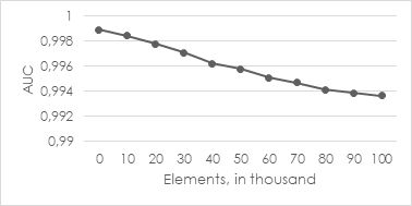
We evaluated the behavior of the online model after supplying it with unseen data points like described above. After every update we measured the AUC value and plotted the AUC trend line on a diagram. Illustration 4 shows the AUC metric dependent on time. We used mini-batches of 10.000 data points for every single update and an unspecified half-life parameter. This means that the model does not “forget“ any data points. One can see that the model quality slowly decreases with every update. One could interpret this result as adaptive behavior on new data points, too.
In comparison to that, let’s consider another example. In illustration 5, one can see the behavior with a configured half-life value of 5.000 elements (which is an extreme example value). So, the model weighs past data instances only half when re-calculating the cluster centers after 5.000 observed elements.
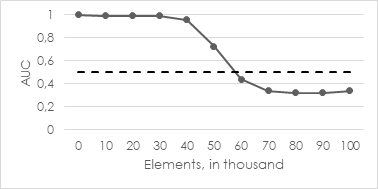
You clearly recognize that the quality of the model drops off over time (after 50.000 new elements). Please note that the black, dashed line shows the baseline for a random, hence useless predictor. We can explain this effect as follows: The contained anomalies suddenly skewed at least one cluster center such that an “abnormal“ cluster emerged. This leads to the fact that the normal data points, belonging to the affected cluster, have a distance longer than the predefined threshold and are therefore classified as anomalies. This leads to a high false positive rate and is expressed by the curve in illustration 5.
Another interesting question was to research the behavior of a corresponding offline model with incremental updates containing the same data as fed into the streaming model. For the offline model we have no half-life parameter for tuning the “forgetfulness“. Instead, we have other options we can tweak, such as the number of iterations over the training data and the initialization method for k-means. Illustration 6 shows multiple different runs of k-means for a different number of iterations with random initialization.


One effect we can observe is that the anomalies have a greater influence on the model with a higher number of iterations (which is pretty reasonable). Another thing we could observe is that the AUC value is “jumping“ up and down while the basic characteristic of the curves remains the same. This suggest that the offline model adapts the actual situation (relation between normal and abnormal data points) most exactly.
Let’s try a special initialization algorithm (k-means || [2]) which finds optimal initial cluster centers before the actual clustering starts. The corresponding results are shown in illustration 7.
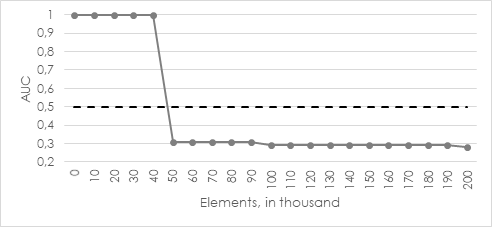
The quality drops off under 0.5 already after the first incremental update set. A variation of the number of iterations haven’t led to another result. So, we can conclude that offline model with k-means|| algorithm adapts the actual dataset (consisting of some normal points and 10 % anomalies) best and finds the optimal cluster centers before clustering at all.
Conclusion and further research
In this blog post we described an experimental set-up for testing and comparing two basically different variants of k-means for anomaly detection with the help of receiver operating characteristics (ROC). A batch/offline model is trained with a predefined, initial training set and then used for predictions. If we need to adapt the incoming data directly (for example if we want to avoid continuously false positives because of a very volatile network environment), we could consider using a streaming/online model.
We were able to show that an online model adapts incoming data points and can be tuned with a so-called half-life parameter. It tunes the “forgetfulness“ of the model. Higher values for half-life lead to a more stable models and less adaption while lower values lead to faster adaption and potentially volatile cluster centers. Without more advanced logic for filtering anomalies before supplying them into the streaming model, such an approach doesn’t give enough control over the behavior of the cluster centers.
On the other hand, we described that a batch-trained model with advanced initialization algorithms (k-means||) adapts much more precise the fed data situation. For the mentioned reasons, in safety-critical use cases like intrusion detection, a batch model is recommended which is updated within controlled times and with preassigned data only. The downside here is, that a mechanism for labeling and checking anomalies is needed beforehand which can filter them out before re-training the model.
We could also compare the training performance (training times) of the both variants as another comparison metric. A presumption is that the online model is much faster in adapting new data points than a total re-training of a batch model. But this has not been further researched in this project.
Sources
[1] Sculley D. (2010): Web-scale k-means clustering. In: Proceedings of the 19th international conference on World wide web. ACM. S. 1177-1178.
[2] Bahmani B.; Moseley B.; Vattani A. et al. (2012): Scalable k-means++. Proceedings of the VLDB Endowment, 5 (7). S. 622-633.