The Internet of Things has proliferated large-scale deployments of devices that continuously monitor changes in their local environment. The data collected by such devices can be leveraged for certain predictive maintenance use cases. In this blog post, we demonstrate how survival analysis can be applied to a real-life predictive maintenance problem using sensor data from IoT devices. We lay out the steps necessary to prepare the data and train several survival models for state of charge (SoC) prediction.
Use Case
Data loggers are IoT devices that continuously monitor the local temperature of industrial refrigerators. The loggers are powered by non-rechargeable batteries, which eventually deplete their charge and require manual replacement. The remaining capacity of the loggers is represented by the state of charge (SoC).
Replacing the batteries when the SoC is low ensures continued functionality of the data loggers. This ad-hoc method of battery replacement is suitable for deployments with a small number of loggers. When dealing with larger deployments, it is often more practical to replace the batteries of all the loggers simultaneously. However, this bulk replacement method cannot take into account the different SoC levels of all the loggers, leading to occasional battery replacements occurring at a high SoC.
This method certainly has room for improvement. If the time when a logger device reaches a low SoC could be predicted, similar time intervals for multiple loggers can be identified. This approach to predictive maintenance results in much easier planning of optimal battery replacement times, saving on manpower and energy costs.
Method
Sounds like a great idea, isn’t it? Easier said than done, though. As some batteries are replaced at a high SoC, these replacement instances cannot be used for training a prediction model. These data are censored, as the time when a low SoC is reached is not seen at all. Dealing with censored data is problematic. Typical machine learning methods cannot handle them. But by leaving out censored data in model building, we risk introducing bias into the resulting predictions.
Fortunately for us, the field of survival analysis is equipped to handle censored data. These statistical methods center around the analysis of so-called time-to-event data. A typical event is death or failure. As the interpretation of survival methods hinges on the specific event that is analyzed, the first step is to define an event for our specific use case.
Defining the Event
To define the event, we first examined the time series data produced by the data loggers. The most prominent variable is the state of charge (SoC) of a data logger over a period of time. As the data was provided by an industrial partner and thus reflects behavior in real-world environments, the SoC of each data logger decreases at different rates with time. An example of the SoC over time for a data logger is shown in Figure 1.
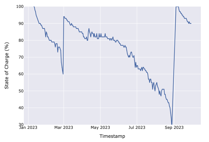
We used an SoC threshold to define the event. Let us illustrate with an example. Figure 1 shows the SoC of a data logger over time. The data logger had its batteries changed in March and September. This is inferred from the sudden spike in the SoC. We define an event to have occurred when the SoC of a data logger reaches 30%. Thus, an event occurred in September, as the data logger reached 30% SoC and subsequently had its batteries replaced. In contrast, the data logger had its batteries replaced at 60% SoC in March. The 30% SoC threshold is not observed. This is censoring, where the data logger “drops out“ before experiencing the event.
Labelling Individual Cycles
After defining the threshold event, we identified the points where a data logger experiences an event or is otherwise censored. To this end, we segmented the SoC curve of each logger into distinct cycles. An event or censorship causes a cycle to end and a new cycle to begin. A cycle can also be defined as the time between battery replacements. Thus, the data logger in Figure 1 has 3 total cycles, 2 of which are censored.
As the cycles were not labeled in the data, we used a peak detection algorithm from the Python Scipy library to identify the starting points of the individual cycles. The algorithm compares neighboring points in a curve to find local maxima. These local maxima correspond to the aforementioned starting points, which are easily visually identified as sharp spikes in the SoC. By marking these points, individual cycles can be segmented.
Extracting Features
Survival analysis methods cannot directly work with time series data. We therefore converted the time series data into a tabular format by computing summary statistics.
These included cycle-specific features, such as the duration and rate of discharge. The rate of discharge is the rate at which the SoC decreases in that cycle. Additionally, the data loggers record their local temperatures in a separate time series. By lining up the timestamps of both the SoC and temperature time series, we extracted the mean temperature in each cycle. Finally, we also included metadata such as the battery type used by the logger from a separate table.
These features are tabulated in a new dataset, where each row represents a cycle.
Fitting an Overall Survival Curve
The labeling and feature extraction steps resulted in a dataset containing the duration of each cycle and a binary variable indicating if the cycle reached the 30% SoC threshold or was censored. The dataset consists of 173 cycles, with 68% of them being censored.
With this information, we proceeded with basic survival analysis using the Kaplan-Meier estimator. The estimator fits a survival function on all the cycles. The survival function is the primary output of survival models, and it expresses the probability of a cycle not reaching 30% SoC at a specific time point.
For each observed point in time, the estimator calculates the ratio of cycles that have not reached the threshold to cycles that are at risk. At-risk cycles have either already reached the threshold at that time, or will reach the threshold or otherwise be censored in the future. As censored cycles remain at risk until they become censored, they can contribute to the estimation of the survival function. For a more mathematical explanation of how the survival function is computed, refer to Kaplan and Meier’s seminal paper [1].

Figure 2 shows the survival function fitted by the Kaplan-Meier estimator. The survival function is steep in the initial 100 days, indicating that a majority of the cycles reach the 30% SoC threshold early. However, there are a few longer-lasting cycles, taking up to 300 days before reaching the 30% SoC threshold. These cycles gradually reach the threshold at discrete times, forming the characteristic step-like curve at later times. The late cycles are presumably due to using high-performance batteries for powering the data loggers.
An important quantity is the median survival time. It is the time when 50 % of the cycles have reached the threshold, and 50 % have not, with respect to censoring. It corresponds to the survival probability of 0.5. The median survival time of the cycles is 255 days. Conversely, the median time to the threshold for exclusively non-censored cycles is 47 days. This large discrepancy in both medians is indicative of the bias that would occur in later modeling when censored data is not taken into account.
Fitting Individual Survival Curves
The Kaplan-Meier estimator (KM) fits a survival function on the whole dataset. To make predictions for individual cycles with unique feature combinations, we require models that can fit survival curves for each cycle. To this end, we chose two models – the Cox proportional hazards (CPH) model and the random survival forest (RSF). The CPH model is a regression model, while the RSF is an extension of the Random Forest model for censored data. For a detailed description of both models and how they fit individual survival curves, refer to Haider et al. [2].
Due to the small sample size, we used only three features when training models. These include the battery type of the logger, the mean temperature of the cycle, and the discharge rate of the previous cycle. The numerical features were chosen by examining their correlation, while the categorical features were chosen by comparing the difference in the survival curves per category.
Next, we split the cycles into train and test sets on the device level, with all cycles belonging to a specific device being assigned to either the train or test set. Thus, all the cycles from 70% of the devices are contained in the train set, and vice versa. The split by device was conducted to avoid potential data leakage, which occurs when cycles from an identical device are present in both the train and test sets.
Evaluation
The performance of both models was evaluated by computing the integrated Brier score (IBS), a variant of the mean squared error for censored data. The closer the IBS is to 0, the better the model. Random models have an IBS of 0.25. As shown in Table 1, all models performed better than random, with the RSF performing the best. This is expected as predictions from the RSF are averaged from an ensemble of trees, leading to a better IBS.
| Model | Integrated Brier Score (↓, 0 ≤ IBS ≤ 1) |
|---|---|
| KM | 0.206 |
| CPH | 0.137 |
| RSF | 0.109 |
The IBS is a standard metric for evaluating model performance for both event and censored cases, but the primary use case for the survival models is to predict the time to the 30% SoC threshold for current cycles. As these cycles have not experienced the event yet, they are considered censored. Therefore, we also examined the predicted survival functions for censored cycles.
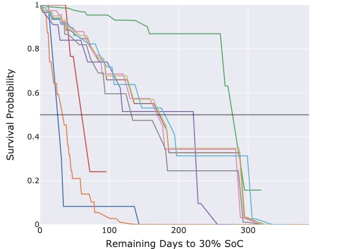
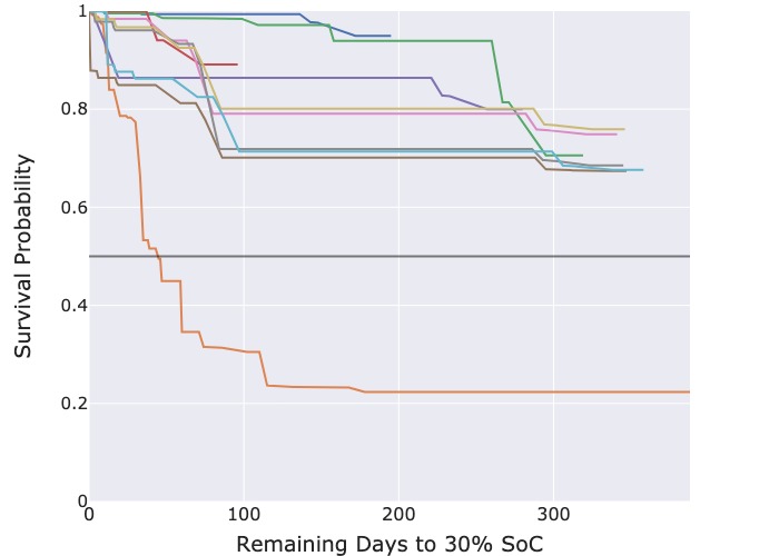
Figure 3: Predicted survival functions for censored cycles.
It is important to emphasize that survival models do not produce point estimates like traditional machine learning models, but instead, output predicted survival functions. These are probability distributions and need to be interpreted accordingly.
Each survival function seen in Figure 3 corresponds to the latest battery cycle of a data logger. As these cycles are the newest, the batteries have not yet been replaced and are therefore censored. Thus, a survival function describes the probability of a logger reaching the 30 % SoC threshold on subsequent days. Replacement times for multiple loggers can thus be inferred by identifying common time intervals with identical survival probabilities for each logger.
The predicted survival functions from the CPH model in Figure 3a deliver useful information as each survival function crosses the probability threshold of 50 %, enabling the extraction of the median predicted survival time. However, those from the RSF model in Figure 3b are overly optimistic. Most censored cycles have a predicted 70 % probability that the threshold event will still not occur even after 300 days.
As the survival curves predicted by the RSF model have overly optimistic and near identical estimates of the median survival time, we concluded that the RSF model is unsuitable for actual deployment for this specific use case. Instead, we recommend the CPH model which generates more realistic survival curves.
Conclusion
To sum up, we used survival analysis methods to generate probabilistic estimates for the time to reach certain state of charge (SoC) thresholds. This approach to predictive maintenance allows planning battery replacement times for multiple data loggers concerning the SoC. To this end, we defined a suitable survival event and processed the time series of the data loggers into a tabular format for training survival models. By interpreting the predicted survival functions, possible replacement times for multiple data loggers can be identified.
What’s next? A possible avenue for future work is a comprehensive evaluation using a larger dataset. As the current dataset had a limited number of cycles, the robustness of the models is questionable. Having more data would let us further explore this line of questioning, as well as test alternative models that would overfit if used on small sample sizes like this dataset. Methods for data augmentation or simulation may come into play here.
Another issue is the interpretability of the generated predictions. Interpreting survival functions requires a background in survival analysis, which not everyone has, especially potential users of the models. A simple solution is condensing the function down to a simple point estimate using the predicted median survival time. However, Henderson and Keiding [3] argued against this approach as it results in a loss of information. Therefore, it is worth conducting a more holistic investigation into the interpretability of the predictions that incorporate user feedback.
These aspects will be further investigated in the DeKIOps research project at inovex. Stay updated for any further developments by keeping up with the blog!
References
[1] E. L. Kaplan and P. Meier, ‘Nonparametric Estimation from Incomplete Observations’, Journal of the American Statistical Association, vol. 53, no. 282, pp. 457–481, Jun. 1958, doi: 10.1080/01621459.1958.10501452.
[2] H. Haider, B. Hoehn, S. Davis, and R. Greiner, ‘Effective ways to build and evaluate individual survival distributions’, J. Mach. Learn. Res., vol. 21, no. 1, p. 85:3289-85:3351, Jan. 2020.
[3] R. Henderson and N. Keiding, ‘Individual survival time prediction using statistical models’, J Med Ethics, vol. 31, no. 12, pp. 703–706, Dec. 2005, doi: 10.1136/jme.2005.012427.