Time series data is part of many real-world applications, e.g., weather records, patient health evolution metrics, (industrial) sensor data, stock prices, website clicks, server metrics, network data, political or sociological indicators, video and voice messages, or shutter speeds – just to name a few. More precisely, a time series is a temporal sequence of arbitrary data, such as a (continuous) series of measurements. The handling of time series requires a precise mathematical framework, which we introduce in this article. If one considers its individual components and their complexity, it becomes clear why dealing with time series data is difficult.
What the heck is a time series?
A time series can be understood as a sequence of (real-valued) random variables generated by a time-dependent system, something that changes over time according to certain rules, also called a dynamical system \((\Omega, \mathcal{A}, \mu, T)\). We get straight into mathematics.
Dynamical system
We start by clarifying the mathematical components of a dynamical system \((\Omega, \mathcal{A}, \mu, T)\) that generates a time series. If you are not interested in maths, I am not mad and you can skip to the first tl;dr, but it helps to understand the challenges of dealing with time series in the next section.
- The set \(\Omega\), also called state space, contains all possible states or more general values of the system. As with non-time-dependent variables, states include latent variables, i.e., difficult or impossible states to measure. For example, one’s income is often also dependent on one’s reputation, which is determined individually by the recruiter and thus cannot be measured.
- Events are taken from a so-called \(\sigma\)-algebra \(\mathcal{A}\) on \(\Omega\). If you are not a mathematician and have never heard this term before, do not worry. It is a mathematical construct that I mention for the sake of completeness but is of no further importance here. Put simply, it collects all combinations and subsets of the possible states (events) that are to be measured, i.e. assigned a probability. Both components together \((\Omega,{\mathcal {A}})\) form a measurable space.
- The measurable space is provided with a special measure, i.e. a probability distribution \(\mu\), which all states \(\omega\in\Omega\) follow. All three components \((\Omega,{\mathcal {A}}, \mu)\) form a probability space.
- Last but not least, the function \(T\) is a map describing the change or dynamics of the system at times \(t\in\mathbb{N}\). At time \(t\) the system is in state \(\omega\), at time \(t+1\) the system is in state \(T(\omega)\) and at time \(t+s\) the system is in state \(T^{\bullet s}(\omega)\), where \(T^{\bullet s} (\omega) := T(\dots T(T(\omega)))\) is the s-fold concatenation of \(T\). Moreover, we assume that the function \(T:\Omega\rightarrow\Omega\) is \(\mu\)-preserving, i.e., for all \(A\in\mathcal{A}\) is \(\mu(T^{-1}(A))=\mu(A)\). This ensures an identical distribution of the states over time, which means that each point in time provides information about the same data-generating process.
To summarize, these four mathematical elements describe a theoretical, dynamic process over time that generates a time series.
Stochastic process
A sequence of random variables or vectors, all defined on the same probability space \((\Omega, \mathcal{A}, \mu)\), is called a stochastic process. In the case of real-valued random variables, a stochastic process is a function
\(\begin{equation} X:\Omega\times\mathbb{N} \rightarrow \mathbb{R} \end{equation}\)
\(X (\omega,t) := X_t(\omega).\)
A stochastic process depends on both coincidence and time. Note that in the most simple case \(\Omega\) matches with \(\mathbb{R}\) and \(X\) with the identity map. Then the observations are directly related to iterates of some \(\omega\), i.e. there is no latency, and the \(X\) itself is redundant.
Time series
Over time, the individual variables \(X_t(\omega)\) of this stochastic process get observed values (expression of a characteristic or several characteristics, observations), so-called realisations \((x(t))_{t\in \mathbb{N}}\). The sequence of realisations is called time series. With the formalism from above and fixing of some \(\omega\in\Omega\), a time series is given by
\((X(\omega), X(T(\omega)),X(T^{\bullet 2} (\omega)),\dots) = (x(t))_{t\in\mathbb{N}}.\)
In many cases, the terms time series and stochastic process are used interchangeably. The subtle difference is shown in Table 1.
| \(t\) fixed | \(t\) variable | |
| \(\omega\) fixed | \(X_t(\omega)\) is a real-valued number | \(X_t(\omega)\) is a sequence of real-valued numbers (e.g. time series) |
| \(\omega\) variable | \(X_t(\omega)\) is a random variable | \(X_t(\omega)\) is a stochastic process |
Table 1: Difference between time series and stochastic processes.
tl;dr
Time series data are a sequence of observations, also called realizations or paths, generated by a stochastic process or in more general by a dynamical system that changes over time. If you want to classify time series data or predict the future, you actually need to gain an understanding of the generating dynamical system, i.e., an understanding of its individual components, i.e., its latent variables, probability distribution, and transition function.
Why dealing with time series is difficult
Why is it so difficult to deal with time series? Why are we not very good at predicting long-term behavior such as the weather or the course of a pandemic like in the case of COVID-19?
Challenges in modeling of dynamical systems
To learn from time series data, i.e., to derive certain properties, classify them, or predict the future, it is actually necessary to know the properties of the generating dynamical system or to model or estimate it as well as possible. In practice, however, we face the challenge that while we can observe data over a longer period of time and thus several over many points in time, we can only observe a few or even a time series sample. In addition, we are also subject to measurement errors or other randomness during the observation process.
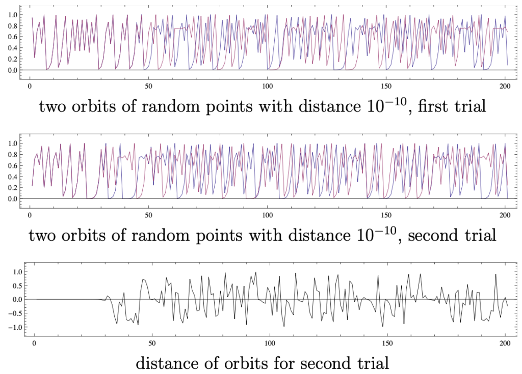
Drawing conclusions from this about the generating system, i.e. about latent variables, distributions, and transition function, is almost impossible because the problem is underdetermined. Even if we can „best estimate“ and model the stochastic process \(X_t\) by data sampling, we rarely have the chance to derive a transition function \(T\) of a dynamical system \((\Omega, \mathcal{A}, \mu, T)\) from only one or a few or even short time series \((x(t))_{t\in \mathbb{N}}\) for purposes of extrapolation. If, on the other hand, one knows the transition function \(T\) or can estimate \(T\) well (as is also indicated in machine learning), one can usually not directly observe the state \(\omega\), i.e. the latent variable. In addition, if one chooses the wrong transition function \(T\), the smallest estimation error of \(\omega\) can lead to the transition function \(T\) causing chaos in the system, as shown in the following example.
An example of chaos and unpredictability: the butterfly effect
Let’s look at a deterministic dynamical system that is an example of how complex, chaotic behavior can arise from a simple transition function \(T\).
Example (Logistic map)
Let \(\Omega = [0,1]\) and for \(r\in[0,4]\) let the transition function of a dynamical system \(T_r:\Omega \rightarrow \Omega\) be defined by
\(T_t(\omega) = r \cdot \omega \cdot (1-\omega),\)
where \(\omega\in \Omega = [0,1]\) models the frequency of the number of individuals in a population in relation to a maximum possible number (resources are limited) and \(r\) is a growth factor. If at time \(t \) the frequency is \(x(t)\), then at time \(t+1\) it is \(x(t+1)=T_r(x(t))\).

‘It can depend on a butterfly’s wing flap in China whether there will be a hurricane in the US some weeks later.’
But that does not always have to be this way. We are not very good at predicting the (long-term) future, but not terribly bad either. In particular, the responsibility for the chaos above lies in the non-linearity of the transition function \(T\). Nonetheless, we should be able to control extreme cases like this, too, if we want to predict the future as well as possible.
By the way: Not all chaos is the same. The Kolmogorov-Sinai entropy offers an interesting possibility to quantify chaos. In the late 1950s, Jakow Sinai succeeded in proving the non-triviality of KS-entropy, in 2014 he received the Abel Prize amongst other things for this. You can read more about entropies in this blog post.
tl;dr
Unlike random variables, time series data depend not only on randomness but also on time. The problem of time series forecasting as an extrapolation problem is extremely challenging, since one only knows the time \(x_t\), but has to estimate the states, i.e. the latent variable \(\omega\), as well as the transition function \(T\). In this respect, the problem is underdetermined and countless different systems could generate the same time series. Even if one specifies the transition function, as one does in machine learning, it is still difficult to determine latent variables. Randomness can also throw a poorly estimated or chosen transition function into chaos, which is why long-term predictions in particular are extremely challenging.
If, on the other hand, one only wants to interpolate well, one has various methods, e.g. from the field of machine learning or from classical time series analysis, which have proven themselves well.
Read more
You are interested in time series prediction? Then the following articles might also be interesting for you:
- Time Series Forecasting with Machine Learning Models: In this article we explain how time series forecasting tasks can be solved with machine learning models, starting with the problem modeling and ending with visualizing the results by embedding the models in a web app for demonstration purposes.
- Hybrid Methods for Time Series Forecasting: Hybrid time series forecasting methods promise to advance time series forecasting by combining the best aspects of statistics and machine learning. This blog post gives a deeper understanding of the different approaches to forecasting and seeks to give hints on choosing an appropriate algorithm.
- TimescaleDB vs. influxDB: Time Series Databases for IIoT: In this article, we discuss our experiences with the two popular open-source time series databases TimescaleDB and InfluxDB. (Article is in German)
References
[1] Karsten Keller, Lecture ‘Chaos and Complexity of Biological Systems’ at the University of Lübeck, summer term 2018.


