Uncertainty Quantification in Deep Learning

Artificial Intelligence—and machine learning in particular—have come a long way since their early beginnings. The widespread availability and affordability of powerful computing resources have enabled the development of complex models like Deep Neural Networks (DNNs). Research has come up with spectacular results in fields like computer vision, speech recognition or game strategies, where Deep Learning has proven to perform as good as or even better than humans in certain scenarios. Learn more about Deep Learning in our blogpost Deep Learning Fundamentals.

How Much Do We Trust Our Models?

Machine learning has found its way into our everyday life in the form of personal assistants like Siri who recognize our desires most of the time. In fact, machine learning has proven to work so well that models are introduced to more and more critical applications. Autonomous driving heavily relies on computer vision based on Deep Neural Networks. Recent EU copyright legislation will require some kind of automatic content filtering, presumably done by machine learning models. And even passport controls will be performed by computers in the future. While we can forgive Siri for making mistakes every now and then, the latter applications require models that are correct one-hundred percent of the time.

While we usually cannot guarantee our models to be absolutely perfect, we could use information about how certain they are with their predictions. That way, in case of high uncertainty, we can perform more extensive tests or pass the case to a human in order to avoid potentially wrong results. This, however, requires our models to be aware of their prediction accuracy for a given input. In the following, we are going to teach Artificial Neural Networks (ANNs) and Deep Neural Networks in particular to do exactly that.

Don’t Mistake Class Probabilities for Confidence

Classification problems are often solved with the help of DNNs, which will return a vector of assignment probabilities (given by a softmax transformation) for the classes being considered. When the probability for one class is considerably higher than the other probabilities, we often interpret this as high confidence. Don’t be deceived!

Consider a DNN that is being trained to distinguish between images of cats and dogs, thus being a classifier with two possible entities. After enough training data, in terms of labeled cat and dog images, has been used to adjust the network parameters, we expect it to do a decent job telling the two kinds of animals apart. Simply speaking, it does so by extracting features that are inherent to the animal (e.g. facial characteristics or fur texture) and assigning them to the corresponding class.

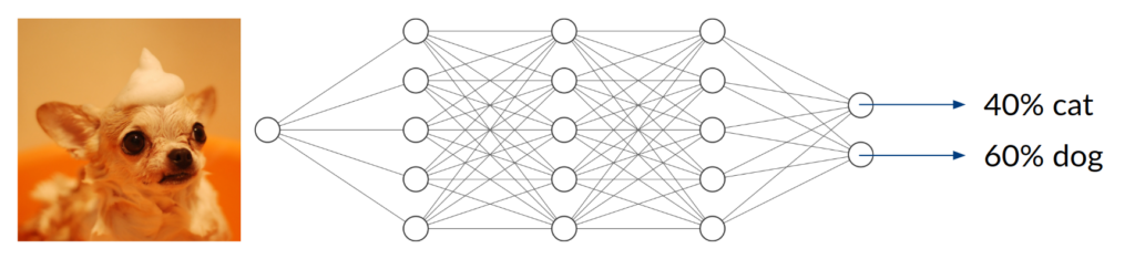
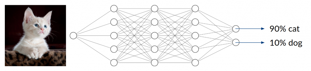
Now, what happens if you take an image of a bird and give it to the trained network to classify? It will most likely not find any characteristic features of cats or dogs. You might think that the network will obviously return something around (50/50) because it can detect neither of the two classes it was trained on. In fact, however, the result could be anything from (0/100) to (100/0). Since the network has never been trained using anything but images of cats and dogs, we don’t have any control over the network’s behavior when given other inputs. This can lead to disastrous misjudgment.

Two Types of Uncertainty

The previous example explains the results of epistemic uncertainty, also called model uncertainty, that is, the uncertainty that results from a lack of training data in certain areas of the input domain. While ANNs perform very good at interpolation tasks, it is adequate to say that they cannot extrapolate. In other words, neural networks can only deal with the things they have seen before. Usually, our training data only covers a very small subset of the entire input space, which means that our trained network will produce arbitrary output values for the vast majority of possible input values. In many applications, this is not an issue as long as we know that future inputs will be similar to the training data. If this is not the case, however, we would like to quantify the lack of accuracy due to missing training data.

On the other hand, we also have to deal with the potential intrinsic randomness of the real data generating process. We call this aleatory uncertainty. As an example, consider the following regression problem. We want to predict the trajectory of an arrow, where the given inputs are the archer’s force when pulling back and two angular dimensions denoting the direction of the shot. The output will be a point on a two-dimensional target. Sounds like a reasonable, deterministic setup? Not so fast! We can safely say that, even with equal force and direction, no two shots will hit the exact same point on the target. This is due to parameters that we do not consider in our model, like wind or air pressure, and unknowns that we simply cannot measure like imperfections in the arrows. As a result, our training data might include samples with identical or very close input values and a whole spread of output values at the same time. We want our model to account for this randomness that is inherent to the data that we are analyzing.

We can further distinguish between homoscedastic and heteroscedastic aleatory noise. Noise is called to be homoscedastic if it follows the same distribution indifferent of the input values. Heteroscedastic noise, on the other hand, depends on the input and can, thus, change in variance or even distribution across the input domain.

Figure 3 shows a very basic data model with one input dimension and one target dimension. The noisy data (black) is generated based on a deterministic mean function (red). The vertical spread for similar input values can be considered aleatory uncertainty. On the other hand, the lack of data on parts of the input domain will result in epistemic uncertainty since the mean function is unknown in practical scenarios.

Methods

In the following, I want to give short and concise explanations of the methods that we use to tackle our problem of uncertainty quantification. For this work, we want to put aside classification problems. Instead, we’ll focus on a very simple regression setup with a single function input and a single function output.

Monte-Carlo Dropout

The Dropout method has been used in ANNs for a long time in order to avoid over-fitting. Network nodes (i.e. neurons) are disabled randomly during training time so that with each training step, a different subset of the network architecture is evaluated and adjusted. This can be seen as a kind of regularization and proves to result in better generalization in many cases.

Monte-Carlo Dropout takes this randomization procedure one step further. Not only do we randomly turn off network nodes for each training step, but we also introduce this kind of randomness to the prediction procedure. This results in a random prediction with some complex probability distribution every time an input value is passed to the ANN. Now, if we apply the same input to the network many times, we can deduce an empirical distribution over the outputs or even estimate parameters for a distribution family like the Gaussian (normal) distribution. The empirical distribution or parameter estimates can then be used to obtain, for example, a mean value and a confidence measure in terms of the distributional variance. We expect that the empirical variance is low where there was an abundance of training data since all network subsets had the opportunity to learn in these areas. However, in areas where there was no training data to learn from, the network behavior is not controllable so we expect a high variance among the different network subsets. This corresponds to our desired behavior for the uncertainty estimation.

Deep Ensembles

Distributional Parameter Estimation

In a general regression setup, the neural network takes a vector of inputs and generates a single output that represents our prediction. This is done according to the network parameters obtained during the training process. However, if we assume our real data to behave according to a parametric probability distribution whose parameters depend on the input values, we can take the underlying model into account and estimate not only the actual output value but a set of distributional parameters.

Assume, for example, that our model has a single output \(y\) which is not deterministic but normally distributed with parameters \((\mu(x), \sigma^2(x))\), depending on the input \(x\). In the training process, instead of using the very common mean squared error (MSE) loss function

\(\mathcal L_{MSE} = \frac{1}{N} \sum_{i=1}^N (\hat{y}(x_i) – y_i)^2,\)

which compares our model output \(\hat{y}(x_i)\) to the real output \(y_i\) for each data pair \((x_i, y_i)\), we must now take into account the distributional variance that we want to estimate along with the mean value. We can achieve this by using a maximum likelihood (ML) approach. We take the negative log-likelihood function of the normal distribution as a loss function, ignoring constants,

\(\mathcal L(x, y) = – \log \phi(y | x) = \frac{\log \hat\sigma^2(x)}{2} + \frac{\left(y – \hat\mu(x) \right)^2}{2\hat\sigma^2(x)}, \)

where, for multiple samples, we average over the log-likelihoods to get the mean negative log-likelihood (MNLL)

\(\mathcal L_{MNLL} = \frac{1}{N} \sum_{i=1}^N \mathcal L(x_i, y_i).\)

Intuitively, the numerator of the second term in the negative log-likelihood function encourages the mean prediction \(\hat\mu(x)\) to be close to the observed data, while the denominator makes sure the variance \(\hat\sigma^2(x)\) is large when the deviation from the mean \(\left(y – \hat\mu(x) \right)^2\) is large. The first term acts as a counterweight for the variance not to grow indefinitely.

This strategy is able to capture the aleatory uncertainty of our data generating process in areas of sufficient training data. While we used a model of normally distributed data in our example, the method can be applied to other parametric distributions in the same way.

Ensemble Averaging

The introduction of parameter estimation enables us to capture distributional information where training data is available. However, the mean, as well as the variance estimations for areas that are not included in the training data, are still uncontrollable. While a sensible mean value might be impossible to find, we would like our network to admit a high uncertainty in terms of a high variance prediction.

Instead of training a single network, we are going to train an ensemble of \(M\) networks with different random initializations. While we expect all networks to behave similarly in areas of sufficient training data, the results will be completely different where there is no data available. For a final prediction, we now take all networks and combine their results into a Gaussian mixture distribution from which we can, again, extract single mean and variance estimations

\(\begin{array} \tilde\hat\mu_c(x) &= \frac{1}{M} \sum_{i=1}^{M} \hat \mu_i(x), \\ \hat \sigma_c^2(x) &= \frac{1}{M} \sum_{i=1}^{M} \hat\sigma^2_i(x) + \left[ \frac{1}{M} \sum_{i=1}^{M} \hat\mu^2_i(x) – \hat\mu_c^2(x) \right]. \end{array}\)

This variance prediction even allows to clearly distinguish between the two types of uncertainty. The first term, denoting an average of all variance estimates, can be interpreted as aleatory uncertainty. The remaining term can be considered epistemic uncertainty, which is low if all mean estimates agree on a similar value and grows if the mean estimates differ widely.

Dropout Ensembles

As an experiment, we combined both Monte-Carlo Dropout and Deep Ensembles and called it Dropout Ensembles. Just like with Deep Ensembles, we estimate distributional parameters instead of actual output values. However, instead of training multiple networks, we train a single network with Dropout. At prediction time, we keep Dropout enabled and generate \(M\) random parameter outputs. These can then be used like actual ensemble outputs in order to obtain a single estimation consisting of mean and variance.

Quantile Regression

Another classic method for distribution estimation is Quantile Regression with neural networks. In this setup, we train a network to estimate quantiles by using the loss function

\(\mathcal L_{QR}= \sum_{i=1}^{N} r_i \cdot \left( \tau – \mathbb{1}_{< 0}\left(r_i\right) \right)\)

where \(\tau\) is the quantile we want to estimate and \(r_i = y_i – \hat q_{\tau}(x_i)\) is the residual of the \(i\)-th sample output with respect to the quantile estimation. It can be shown that, in expectation, the loss function is minimal when the true quantiles are returned, which motivates the use in a neural network.

Now, we only need to estimate two different quantiles in order to infer a specific Gaussian distribution. Again, this distribution can be used to estimate confidence by taking the standard deviation parameter.

Gaussian Process Inference

A Gaussian Process is a random function, which is defined by its mean and covariance functions. Now, taking a finite set of function inputs, the output values will always behave according to a multivariate normal distribution with parameters taken from the (input-dependent) mean and covariance functions. Thus, a Gaussian Process can be considered a multivariate normal distribution with \(\mathbb R\)-infinite dimensions.

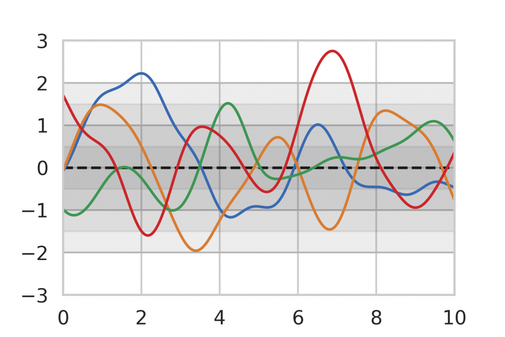
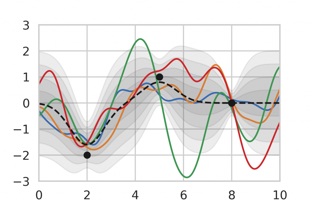
As a baseline for our method evaluation, we included Gaussian Process inference, which is an analytic method for Bayesian Inference on functions. The general idea of Bayesian Inference is to assume a prior distribution that represents the knowledge before any data points have been seen. An example can be seen in Figure 8 where we limit ourselves to the assumption that our function is a Gaussian Process, centered around the mean (dashed line) 0 with a certain variance (shown as gray shades). The colored lines show random realizations of the Gaussian Process.

After being given a set of data points, we can use the analytic inference formula for Gaussian Processes to calculate the posterior distribution. In Figure 9, we observe that the posterior mean is drawn towards the observations and the variance decreases in the vicinity. Note also that the variance is lower for data points that are observed multiple times (right) compared to single observations (left, middle). This corresponds to our intuition of how inference should behave, which motivates the use of Gaussian Process inference as a baseline.

Unfortunately, Gaussian Processes do not scale very well with large amounts of data. The complexity of our inference formula is \(\mathcal O(n^3)\), which makes it infeasible for big data applications. Also, Gaussian Processes require a lot of preliminary thought and assumptions about the data. For more details about the Gaussian Process setup, please refer to my thesis.

Evaluation

For the analysis of the methods proposed, we use a very simple model. We consider a univariate (1-dimensional input) real-valued (1-dimensional output) function \(f\) as a basis. We create synthetic data as a combination of the deterministic function and homoscedastic Gaussian noise:

\(y_i = f(x_i) + \epsilon_i, \quad \epsilon_i \sim \mathcal{N}( 0, \sigma^2)\)

Our input values, \(x_i\) are random, uniform draws from the interval \([0,10]\). The Gaussian noise represents our intrinsic aleatory uncertainty since it is part of the data-generating process. Figure 10 shows random data points along with their mean value and a band of five standard deviations.

For our test setup, we use a comparably shallow network consisting of two hidden layers, each containing 20 nodes using ReLU non-linearities. Our Deep Ensembles consist of 5 networks. Training is performed using Adam optimizer with a batch size of 128 and early stopping. At prediction time, Monte-Carlo Dropout and Dropout Ensembles take 100 samples for their estimates. For all networks, learning rates and weight decay factors are optimized. The dropout probability for Monte-Carlo Dropout and Dropout Ensembles are also subject to optimization.

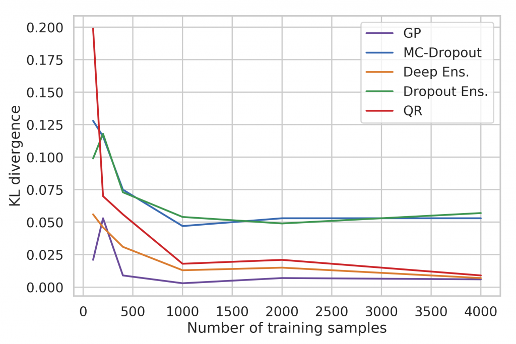
In order to compare the estimation qualities, we need a suitable criterion. One possible choice is the Kullback-Leibler (KL) divergence, which quantifies the distance of two distributions. The KL divergence between two Gaussian distributions, for example, is given as

\(D_{KL}(P \;\|\; Q) = \log\left(\frac{\hat\sigma}{\sigma}\right) + \frac{\sigma^2 + (\mu – \hat\mu)^2}{2\hat\sigma^2} – \frac{1}{2}.\)

Figure 11 clearly shows the relation between the number of training samples and estimation accuracy. Naturally, the quality increases with the amount of training data while the training time increases as well. We can see that Deep Ensembles, Quantile Regression, and Gaussian Processes can benefit from a large training set while the accuracy of the Dropout approaches is limited due to the intrinsic noise being introduced by the Dropout procedure.

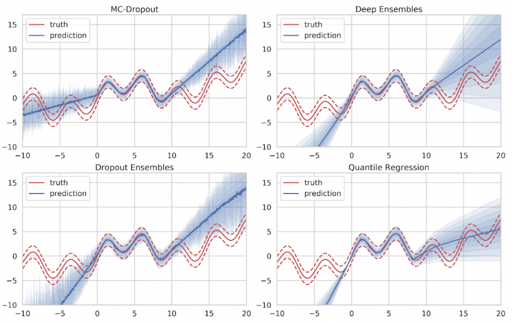
Looking at the actual estimates in Figure 12, we can see that all approaches produce decent results in areas of sufficient training data. The mean prediction is given by the solid line while the uncertainty prediction is given as blue shades where one shade denotes half a standard deviation. Ideally, the five uncertainty shades will conincide with the variance bands (dashed red). The mean value, as well as the intrinsic aleatory uncertainty, are captured well. However, none of the methods is able to express sufficient doubt in areas where no training data was provided.

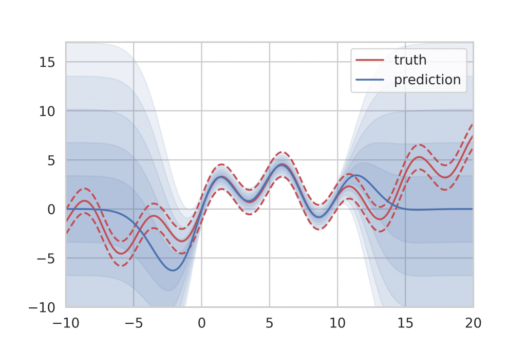
If we take the result of Gaussian Process inference to compare, we can see that Gaussian Processes provide a very clear indicator of ignorance. When no training data is available, they simply fall back to their specified prior distribution, which is easily recognizable at both ends of the training data spectrum in Figure 13. However, Gaussian Processes do not scale very well with large amounts of training data since the inference time is in cubic relation to the number of training samples. This makes Gaussian Process inference infeasible for big data applications.

Additional experiments using synthetic data with heteroscedastic Gaussian noise and non-Gaussian noise show that Deep Ensembles generally produce the best results among the neural network-based approaches. Also, Deep Ensembles, as well as Dropout Ensembles, provide the benefit of being able to separately determine aleatory and epistemic uncertainty. An example of this can be seen in Figure 14 where aleatory uncertainty is denoted by the blue shades and epistemic uncertainty is shown in red shades.

Conclusion

We have shown that it is generally possible to teach Deep Neural Networks to express their prediction uncertainty. All methods being considered are able to reliably determine aleatory uncertainty when given enough training data. However, we have also seen that our neural network based approaches have trouble admitting their ignorance for inputs that have not been included in the training data range. They cannot provide a clear indicator like Gaussian Process inference, which on the other hand does not scale well with the size of the training set. Experiments in various scenarios, e.g. homoscedastic, heteroscedastic and also non-Gaussian noise, have shown that Deep Ensembles and Dropout Ensembles both provide decent results while also being robust in terms of the noise distribution. Furthermore, they are able to differentiate between aleatory and epistemic uncertainty. This could be used to specify a threshold value for only the epistemic uncertainty in order to detect model ignorance.

In the future, trust in our models will be essential for them to be accepted in critical applications. Our approaches for uncertainty quantification in Deep Learning take one first step and provide an objective criterion that enables us to make assumptions about the prediction quality of our model. This will not only make us feel more comfortable using predictions with high confidence measures. It will also give us hints about where our models need more training in case of low confidence measures.

Sources

[1] Uncertainty Quantification in Deep Learning (Simon Bachstein)

[2] Dropout as a Bayesian Approximation: Representing Model Uncertainty in Deep Learning (Yarin Gal, Zoubin Ghahramani)

[3] Simple and Scalable Predictive Uncertainty Estimation using Deep Ensembles (Balaji Lakshminarayanan, Alexander Pritzel, Charles Blundell)