Using Survival Analysis for Cost Optimal Maintenance

In this blog post, we first show what kind of survival data is required for training survival models. We then show how survival models utilize the collected information about the lifecycle of machines to estimate an optimal replacement time for machines experiencing different wear, depending on their operating conditions.

What we cover in this blog post

• • What does a survival analysis dataset typically look like?
  • Fitting Kaplan-Meier estimators on survival datasets
  • Fitting Weibull distributions on survival datasets
  • Fitting Survival regression model (AFT)
  • How to use survival functions to estimate a cost-optimal maintenance cycle

With the advent of big data technologies, many manufacturers and users of industrial machines started collecting data about the lifecycle of their machines. Given that data, methods for analyzing the time it takes for a machine to fail can be used for optimizing maintenance schedules. In this post, we show how numerical estimations, probability distributions, and (survival) regression can be used to calculate the optimal replacement time for wearing parts in machines.

Reactive vs. Preventive vs. Predictive Maintenance

Failure of a part in a complex machine can lead to quality issues or even total failure of the machine. The downtime, or even just the loss in quality, is very costly for those relying on the machines. This is why reactive maintenance (repair only after a part fails) is often not a preferred paradigm. On the other hand, scheduling preventive maintenance at the right time is no trivial task, and without considering the operating conditions of the machines scheduled maintenance is often ineffective if the maintenance cycle is too long, or wasteful and expensive if the maintenance cycle is too short.
In contrast, approaches for predictive maintenance seek to answer the question: When is the optimal time to repair a specific part or a machine considering the operating conditions and the state of the machine?

With the advent of big data technologies, many manufacturers and users of industrial machines started collecting data about the lifecycle of their machines. Modern IoT devices also collect various kinds of runtime and sensor data that can be used to quantify the usage of any particular machine.

Survival Data

As a working example, we use survival data consisting of survival time in days, a censorship indicator, a continuous feature indicating the average usage per day, and a categorical feature indicating the generation of the part. The idea behind the generation label is that parts for machines are oftentimes improved over time. Here we simulate two distinct generations of a part and we expect the generation to have an impact on its durability.
The data was generated using the R library survMS. The dataset contains 1.000 data points, 500 from each generation. The feature daily_usage_h is normally distributed around 9h per day, with a standard deviation of 3h. You can download this data here.

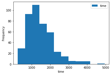
The time column contains the number of days until observation time. At the observation time either a failure had happened (event is True) or no failure had happened yet (event is False).

As a continuous feature, we also collected the average daily usage of the device. Oftentimes, how much a device is used daily has some impact on the time until a wearing part fails, so we plan to use this feature to make our model more accurate.

What is censored data?

Why do we need the ‚event‘ label in our data? When we are working with lifetime data (of humans or machines), there are multiple reasons why we might not have the complete picture. The original motivation for performing survival analysis was literally a matter of life and death. When medical trials are performed on a group of humans, the researchers have to terminate the study at some point in order to publish the results. At that point, a statistically sound analysis of the effect of the medication was required. But the only information the researchers have about the patient that survived at the end of the study was that they survived at least to the end of the study. In long-lasting studies, some participants may leave the study prematurely, for example, because they die in an accident. It would be wrong to attribute these cases to the disease being researched.
In IoT projects, machines are continuously monitored. If we are interested in the failure of a part in a machine, there are several possible reasons we might lose track of this part. Most commonly we lose track of a part because it is being replaced during scheduled maintenance without actually failing. Chances are, you are trying to analyze data from machines that have been in use for several years. It would be wrong to assume that every replaced part in these machines has actually failed.
The event label is used in approaches for survival analysis to distinguish between survival data, where we have actually observed the event we are interested in, and data points where we only know that the individual lived at least this long without experiencing the event.

What actually is a survival function?

The survival function gives the probability that a device survives past a given point in time. It, therefore, is another way of looking at an underlying probability distribution of the survival times observed in our data. The survival function can be estimated using numerical methods like Kaplan-Meier or more sophisticated approaches like distribution-based models or survival regressions. In the rest of this blog post, we guide you through fitting survival models with different methods.

Numerical Survival Analysis using Kaplan-Meier

To get a clearer picture of the data, and for comparing the two generations to each other, we can use a simple tool for survival analysis: the Kaplan-Meier Estimator. In essence, the Kaplan-Meier Estimator iterates over a set of the survival times sorted by the survival time and plots for each point in time the percentage of the population that has survived until this point in time. Censored entries are handled differently, by simply excluding them from the population, but not counting them as failures.

Because we are interested in comparing the survival likelihood of parts from the two generations in our dataset, we split the dataset into two generations and fit a Kaplan-Meier estimator to the two populations.

The result is two estimations for the survival functions of the two generations of the part we are investigating. We can easily see that the newer generation of the part is more durable, and parts of this generation last (on average) slightly longer. This plot can already be used for a ballpark estimation of a preventive maintenance interval. But, this estimation would only take the generation into account, and actually optimizing the maintenance interval for cost would be rather challenging.

Fitting Weibull Distributions to Survival Data

Another approach for finding the survival function of our devices is to fit a probability distribution to the survival times directly while still taking censorship into account, and then deriving the survival function from the probability function to fit the data.
The most common type of distribution used in this application are Weibull distributions. Weibull distributions are so useful because they can take very different forms based on the shape parameter beta. This allows them to accurately model various different kinds of survival behavior seen in practical applications (such as infant mortality or gradual wear).

We use the python library ‚reliability‘ to fit three Weibull distributions to our survival data. One distribution will model the overall survival behavior of all machines in our data. As with the Kaplan-Meier estimator above, we also fit a distribution for only generation one and generation two.

The resulting objects represent Weibull distributions. We can use these objects to plot several derived functions, such as the survival function.

As we can see, the survival functions of the fitted distributions for generation one and generation two match the purely numerical estimation of the survival functions we obtained from the Kaplan-Meier estimator. But, the distributions we fitted to our data give us a mathematically easy (just two parameters) model of the data, that we can use in several applications.

Estimating Optimal Replacement Times

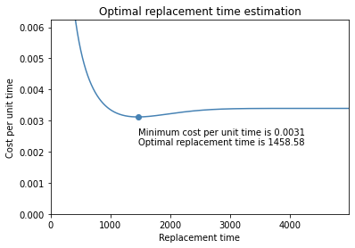
One application that is directly supported in the reliability library, is to find the optimal replacement time. This requires us to supply a simple cost model consisting of the cost of preventive maintenance and the cost of reactive maintenance. In practice, finding these costs can be very challenging. Some considerations that might go into defining these costs may be the cost of the downtime of the machine, required express delivery costs, or additional personal costs required for diagnosing the fault in case of reactive maintenance.
The idea behind finding the optimal replacement time is that the total costs across a range of possible replacement intervals will be higher at the extreme ends of that range. If we decide to replace a part too early, we will have higher costs due to frequent preventive replacements. If we decide to wait too long, the risk of a failure goes up and so do our overall costs, because we will have more reactive replacements.
The fitted distributions give us all the information we need to accurately assess the risk of failure and minimize our overall maintenance costs. In this example, we assume preventive costs of 2.5 units and reactive costs of 5 units.

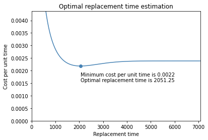
We can clearly see that some improvements have been made to our part in generation two. The estimated optimal replacement time for parts of generation two is a lot longer than in generation one (2.051 days instead of 1.458 days). This also shows that it is important to separate the two generations since the optimal replacement time estimated when not splitting the data lies in between the two estimates for each generation. A replacement interval of 1.891 days would likely be too long for generation one, but too short for generation two.

Problem: We can not easily use features like usage per day!

Because we are completely ignoring the usage per day we observed in our data, the results of this analysis are biased. The specific bias we are subject to in this case is known as the omitted-variable bias. By completely omitting the usage per day and only splitting our population into the two generations, our model attributes all variance in survival rate to just the difference between the two generations.
If we try to take a continuous feature like ‚daily_usage_h‘ into account in a similar way we used the generation, by defining one (or multiple) cut-off points to split the population into smaller groups, we are likely to run into problems.
First, we would need to define a cut-off point. In our example data, we have already seen that the daily usage is normally distributed. Because of this, we might be tempted to define the mean of that distribution (about 9h per day) as a cut-off point and split the population into high and low usage parts. But by defining a cut-off point, we introduce assumptions into our analysis that might not be true. We would assume that a part that is used 30 minutes per day experiences the same wear as a part that is used 8,5h per day.
We could define more cut-off points and split our population into smaller parts, but we have very few observations at the far ends of the daily usage distribution, so our results for these parts are not going to be very accurate or meaningful.

Survival Regression with Weibull AFT

To finally take additional features in our data into account, we take a look at accelerated failure time (AFT) models. The idea behind AFT models is that features collected in the data have an accelerating effect on the mechanical process causing the part to wear and fail eventually. In our example, we can view both the generation of the part and the usage of the machine per day as features that have an accelerating effect on the wear.
We go back to the lifelines library to fit a Weibull AFT to our data. To ensure that the categorical variable ‘generation’ is interpreted correctly, we separate our data set into the two generations again. We then specify the time and event column to indicate the target variable and censorship indicator, respectively. The WeibullAFTFitter then interprets all other columns (in this case only the column ‘daily_usage_h’) as additional features that can have an accelerating effect on the wear.

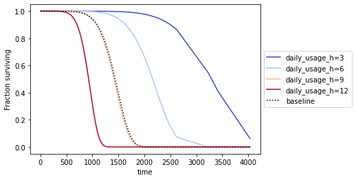
We can then take a detailed look at the partial effects on the outcome that the model attributes to the daily usage for both generations.

We can see that our AFT models consider daily use of around 9 hours as a baseline for both generations. This is not surprising, since it is the mean of the daily usage distribution. A lower-than-average daily usage (e.g. 6 or 3 hours) stretches the survival functions to the right, indicating slower wear.
We can also see that the proportional effect of daily use on the estimated survival time is much greater than the difference between the two generations. The baseline for the first generation at around 9 hours of daily use predicts a 50 % survival rate at around 1.500 days of total use. The same baseline for generation two predicts a 50% survival rate at around 2.000 days of total use. Compared to this the spread in predicted survival rates caused by just three hours of daily use is much greater, regardless of the generation of the part.
We can make this even clearer, by predicting a few survival functions for example devices, and plotting them in the same graph.

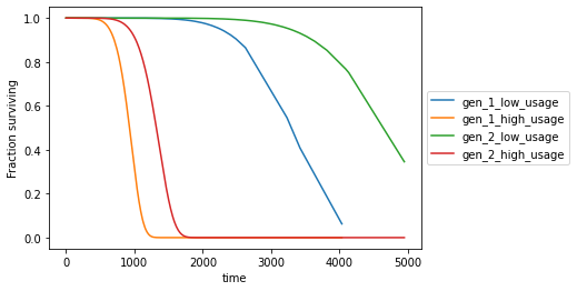
This plot makes it very clear that ignoring the daily usage of the device in our model is detrimental. The difference in expected survival time due to daily usage is a lot bigger than the difference due to the generation.

AFT models come with a few downsides to be aware of. For one, AFT models can only model linear relationships between the different features. Another issue can be features in the data that do not have a meaningful impact on the survival times we are trying to predict. Both of these downsides can be addressed by other types of models, such as Random Survival Forests.

However, we already saw one advantage AFT models have over Random Survival Forests: interpretability. We were able to easily see the effects that both the generation and the daily usage have on the predictions. And because the results of the predictions are essentially Weibull distributions, we can use the predicted alpha and beta parameters of a machine to calculate the optimal replacement time as discussed earlier.

Pitfalls

While all of this works great on generated test data, real-world applications are full of pitfalls to look out for.
Depending on the part you analyze and the domain you are working in, the data that has been collected may not only contain part failures due to wear. There may be accidental failures that are not due to wear, but for example due to user error or other external factors. These failures would still be recorded in the data, but they do not belong to the distribution we are trying to find in the data.
Another very common problem is that the survival behavior may not be as straightforward as in the example illustrated here. A common pattern is a bathtub curve in the rate of failure. Parts may commonly fail early in their life (infant mortality). The rate of failure then goes down, as only robust parts stay in use, until the effects of wear set in, meaning that the rate of failure rises again. Situations like this can be captured by mixture models that can model multiple different distributions in the data.
Sometimes, production-related issues lead to defective subpopulations in the total population of machines you analyze. Identifying these subpopulations can be tricky, but it would be wrong to just fit a single distribution to all of your data because the failures observed in a defective subpopulation can not be generalized to all your devices.
In this blog post, we have worked with synthetic survival datasets including censored and non-censored data. We have shown how to fit numerical survival models. Furthermore, we have shown how to use features in survival models using the survival regression method AFT. Most importantly we have shown how survival models can be used in finding a cost-optimal maintenance cycle.

What we did not cover

We have mentioned that one of the pitfalls of the AFT regression models is their weakness in handling nonlinearity in the data and that random survival forests can handle such data more effectively. In our second blog post, we will guide you through applying random survival forests in python on nonlinear survival data with a large number of features.