Accurate forecasting of electricity consumption is greatly beneficial to companies aiming to achieve efficient and optimized cost management. The key lies in understanding and interpreting respective time series data – a collection of energy consumption measurements recorded at evenly spaced intervals. Analyses and forecasting of time series offer valuable insights into past patterns, trends, periodic fluctuations, and future developments of electricity usage. These insights empower informed decisions regarding resource management.
In this context, statistical and algorithmic approaches are used to ground forecasts on historical data. In recent years, numerous forecasting models have been developed, each leveraging distinct assumptions about the underlying patterns in time series data. Depending on these patterns, the resultant models are suitable for specific applications.
In this blog post, we will take a closer look at a modular regression model called Prophet as a promising model for time series analysis. The investigated time series of energy consumption shows regular seasonalities, and huge trend changes due to external factors or holiday effects. Throughout this blog post, we will detail the process of applying the Prophet model to such data and ascertain its efficacy.
The objective is to develop an implementation that can be applied to a wide range of different energy consumption data. Thus, we will also emphasize an evaluation strategy that is helpful to evaluate multiple time series. This approach facilitates the development of promising performance conditions for Prophet.
Disclaimer:
The content of the blog post assumes familiarity with machine learning concepts, and readers are advised to have a solid understanding of time series concepts for optimal comprehension.
What is Prophet?
Constructing time series forecasting requires a sophisticated set of methods to capture the complex patterns of time-dependent data. In 2017, researchers from Facebook presented their open-source project named Prophet, a framework tailored for modeling time series in Python or R. in their paper “Forecasting at Scale“. It stands out for its user-friendly simplicity and is purpose-built to deliver precise time-series predictions. The intuitively interpretable parameters make it easy to use and understand, even by non-technical analysts.
Derived from typical patterns in characteristically known business time series, it decomposes the time series into three distinct components:
- The trend component covers the general course of the time series, i.e. the non-periodic fluctuations. It captures how the values increase, decrease, or remain constant over time.
- The seasonal component detects recurring seasonal patterns, such as daily, weekly, or yearly cycles.
- The holiday effects component takes important holidays or events that could affect the time series into account.
Prophet is an additive model that considers the sum of these components plus a normally distributed error term. Several other features of Prophet, like efficient and fast training, easy tweaking of hyperparameters, and robust handling of missing records or outliers, make Prophet an appealing time series modeling framework – especially if the application of several time series recorded by multiple different monitoring stations is required. The documentation of Prophet can be found here.
Use case: Electricity consumption forecasts for multiple monitoring stations
In the given scenario, we have measurements available from several measuring points denoted as \(M\), all within the same time period within the identical time period \(0,1,…,T \). Each measuring point \(m\) from the set \(M\) is represented by a time series \(x_m(t), m \in M, t \in \{0,1,…,T\}\). The goal is to predict future measured values for each time series using the prophet model, denoted as \(y_m(t)\) aiming to get as close as possible to \(y_m(t) \approx x_m(t)\) for \(t>T\), \(m \in M\).
The primary aim is to determine a model configuration, which involves model parameters denoted as from a set of potential parameters represented by \(\Omega\). This configuration should incorporate appropriately selected seasonal patterns, holiday effects, and other hyperparameters, aiming to minimize the discrepancy between \(y_m(t)\) and \(x_m(t)\) for \(\omega \in \Omega\). The forecasts of Prophet can show variations in their predicted values for a specific time series based on a used parameter setting. The model is trained on a part of the time series, the so-called training data. After training the model, the difference between unseen values and their predicted counterparts is considered to compute various error statistics. This part of the time series is called validation data. Each error metric quantifies the accuracy of the forecast performance and provides ideas on which parameter setting works best.
Prophet’s Hyperparameter Tuning
Prophet offers cross-validation functionalities to quickly and easily find the best working forecast model across various hyperparameters. It utilizes the so-called simulated historical forecast. The simulated historical forecast is based on a rolling origin evaluation procedure for assessing the quantitative performance of time series forecasts.
For this purpose, \(k\) cut-off points are determined while ensuring that the forecast remains within the historical data. A model is fitted up to a certain cut-off point. Subsequently, predicted values are compared to actual values within the chosen horizon. Iterating across all cut-off points and calculating the average of all computed error metrics, a comprehensive understanding of the forecast performance over time is attained.
Problems faced with Prophet’s Hyperparameter Tuning
In our application case, we need to deal with numerous time series \(x_m, m \in M\). Our goal is to identify a parameter setting \(\hat\omega \in \Omega\) for a single Prophet model that fits all these time series as best as possible, e.g. this model with parameter settings \(\hat\omega\) ensures a reasonable forecast performance for all these time series recorded by the measurement points \(M\). We assume that the time series of the measurement points \(M\) represent the unseen target data in their characteristics.
Due to high manual analysis efforts, individually evaluating each time series using Prophet’s cross-validation is an inefficient method. In addition, Prophet’s cross-validation neglects the effect of the training dataset’s size to which the model is fitted. This plays a crucial role in avoiding overfitting and also addresses the question of how much data must be recorded before running into a cold-start problem.
Alternative evaluation strategy using Prophet for time series analysis
An alternative approach would be to extend the cross-validation by leveraging similar observed patterns of all time series. For this purpose, observations are collected in advance through a deep data analysis, concerning holiday effects, seasonalities, and trend changes at certain changepoints. Also, the amount of historical data on which the model is fitted should be considered.
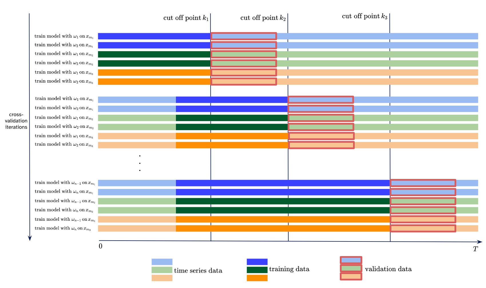
Analogously to Grid Search, the cross-validation loop involves all combinations of collected values for the different observed criteria on different selected cut-off points. Pursuing this evaluation strategy results in \(k* |M| *|\Omega|\) experiments where \(|\Omega|\) denotes the number of all different parameter combinations, and \(|M|\) is the number of all measurement points. A reduction of the number of experiments is achieved, by first starting to cross-validate single criteria. After figuring out appropriate criteria values, a final down-sized cross-validation loop can be implemented. Each experiment resembles different error statistics.

The figure depicts an illustration of the explained cross-validation strategy. Each distinct time series \(x_{m1}, x_{m1}\) and \(x_{m3}\) with \(m1, m2, m3 \in M\) is evaluated on different cut off points \(k_1, k_2\) and \(k_3\), each subjected to various parameter settings \(1, 2, \ldots , n\) and differing sizes of training data.
In the next step, computed error statistics provide the foundation for determining a suitable parameter setting. Further, it reveals in-depth findings about the present time series. It is important to consider an error statistic like the mean average percentage error to ensure comparability between the forecast performances of different time series. In addition, a baseline should also be established that is trained at each cut-off point. Without much implementation effort, Prophet’s default setting can be used for this purpose.
Analysis of error statistics and plots
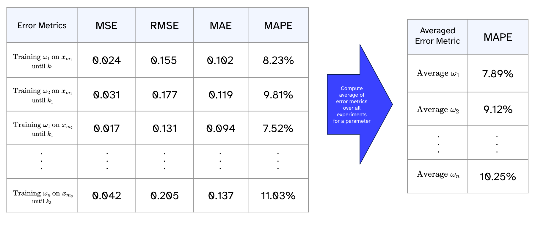
Analyzing the produced error statistics and forecast plots, we can deduce the optimal parameter setting. And even more important, the analysis can be tailored to desired needs. In our described application case, we are interested in a parameter setting that fits all time series well. This entails a comprehensive assessment of averaged error metrics for the considered parameter setups. Thus, the average of error metrics across all cut-off points and each time series is an initial insightful indicator. The following table shows an example of this calculation.

Delving into the averaged performances across different cut-off points might uncover unnoticed weaknesses within certain time intervals. Looking at the averaged performances for individual time series might clarify questions like what makes successful prediction difficult on these data.
Before choosing a certain parameter setting, an individual examination in this particular setting for each time series is essential as well.
Experiences using Prophet as a forecasting model for electricity consumption
Despite computational costs to generate the error statistics for all different combinations of parameters, it is a fast method to develop a sense of what works effectively for forecasting. Furthermore, it reveals any potential issues. Overall it strengthens the understanding of the patterns and characteristics in the time series analysis. The verification by reviewing other parameter settings involving other factors like the training data size, seasonalities, and holiday effects also provides certainty that various options have been thoroughly explored.
We experienced that Prophet’s default parameter setting already performs remarkably well on several time series. So it represents a worthy initiation for prototyping. We further noted that the inherited seasonalities capture underlying fluctuations well. No adaptation for the seasonality effects was required. Moreover, we observed that the inclusion of holidays can be highly beneficial if a global pattern is observed across all available time series.
While it may yield satisfactory results for many time series, it should be noted that it will not achieve the best possible forecasts for every individual time series. Each time series has its own characteristics, possesses outliers, and might be affected by individual external factors. It needs to be acknowledged that a global evaluation over several time series – even stemming from the same domain – does not replace a dedicated analysis for a single time series.
Overall, Prophet’s ease of interpretation and the relatively small number of adjustments to its default hyperparameters contribute positively to its appeal and make it a strong choice for forecast applications in the electricity consumption context.


